Worked Examples from Introductory Physics
(Algebra–Based)
Vol. I: Basic Mechanics
David Mur dock, TTU
October 3, 2012
2
Contents
Preface i
1 Mathematical Concepts 1
1.1 The Important Stuff . . . . . . . . . . . . . . . . . . . . . . . . . . . . . . . 1
1.1.1 Measurement and Units in Physics . . . . . . . . . . . . . . . . . . . 1
1.1.2 The Metric System; Converting Units . . . . . . . . . . . . . . . . . . 2
1.1.3 Math: You Had This In High School. Oh, Yes You Did. . . . . . . . . 3
1.1.4 Math: Trigonometry . . . . . . . . . . . . . . . . . . . . . . . . . . . 5
1.1.5 Vectors and Vector Addition . . . . . . . . . . . . . . . . . . . . . . . 5
1.1.6 Components of Vectors . . . . . . . . . . . . . . . . . . . . . . . . . . 6
1.2 Worked Examples . . . . . . . . . . . . . . . . . . . . . . . . . . . . . . . . . 8
1.2.1 Measurement and Units . . . . . . . . . . . . . . . . . . . . . . . . . 8
1.2.2 Trigonometry . . . . . . . . . . . . . . . . . . . . . . . . . . . . . . . 10
1.2.3 Vectors and Vector Addition . . . . . . . . . . . . . . . . . . . . . . . 14
2 Motion in One Dimension 19
2.1 The Important Stuff . . . . . . . . . . . . . . . . . . . . . . . . . . . . . . . 19
2.1.1 Displacement . . . . . . . . . . . . . . . . . . . . . . . . . . . . . . . 19
2.1.2 Speed and Velocity . . . . . . . . . . . . . . . . . . . . . . . . . . . . 19
2.1.3 Motion With Constant Velocity . . . . . . . . . . . . . . . . . . . . . 20
2.1.4 Acc eleration . . . . . . . . . . . . . . . . . . . . . . . . . . . . . . . . 20
2.1.5 Motion Where the Acceleration is Constant . . . . . . . . . . . . . . 21
2.1.6 Free -Fall . . . . . . . . . . . . . . . . . . . . . . . . . . . . . . . . . . 22
2.2 Worked Examples . . . . . . . . . . . . . . . . . . . . . . . . . . . . . . . . . 23
2.2.1 Motion Where the Acceleration is Constant . . . . . . . . . . . . . . 23
2.2.2 Free -Fall . . . . . . . . . . . . . . . . . . . . . . . . . . . . . . . . . . 24
3 Motion in Two Dimensions 33
3.1 The Important Stuff . . . . . . . . . . . . . . . . . . . . . . . . . . . . . . . 33
3.1.1 Motion in Two Di mensions, Coordinates and Displacement . . . . . . 33
3
4 CONTENTS
3.1.2 Velocity and Acceleration . . . . . . . . . . . . . . . . . . . . . . . . 34
3.1.3 Motion When the Acceleration Is Constant . . . . . . . . . . . . . . . 35
3.1.4 Free Fall; Projectile Problems . . . . . . . . . . . . . . . . . . . . . . 36
3.1.5 Ground–To–Ground Project ile: A Long Example . . . . . . . . . . . 36
3.2 Worked Examples . . . . . . . . . . . . . . . . . . . . . . . . . . . . . . . . . 39
3.2.1 Velocity and Acceleration . . . . . . . . . . . . . . . . . . . . . . . . 39
3.2.2 Motion for Constant Acceleration . . . . . . . . . . . . . . . . . . . . 40
3.2.3 Free –Fall; Projectile Problems . . . . . . . . . . . . . . . . . . . . . . 41
4 Forces I 49
4.1 The Important Stuff . . . . . . . . . . . . . . . . . . . . . . . . . . . . . . . 49
4.1.1 Introduction . . . . . . . . . . . . . . . . . . . . . . . . . . . . . . . . 49
4.1.2 Newton’s 1st Law . . . . . . . . . . . . . . . . . . . . . . . . . . . . . 50
4.1.3 Newton’s 2nd Law . . . . . . . . . . . . . . . . . . . . . . . . . . . . 50
4.1.4 Units and Stuff . . . . . . . . . . . . . . . . . . . . . . . . . . . . . . 51
4.1.5 Newton’s 3rd Law . . . . . . . . . . . . . . . . . . . . . . . . . . . . . 51
4.1.6 The Force of Gravity . . . . . . . . . . . . . . . . . . . . . . . . . . . 52
4.1.7 Other Forces Which Appear In Our Problems . . . . . . . . . . . . . 54
4.1.8 The Free –Body Diagram: Draw the Damn Picture! . . . . . . . . . . 56
4.1.9 Simpl e Example: What Does the Sc al e Read? . . . . . . . . . . . . . 56
4.1.10 An Important Example: Mass Sliding On a Smooth Inclined Plane . 58
4.1.11 Another Important Example: The Attwood Machine . . . . . . . . . 61
4.2 Worked Examples . . . . . . . . . . . . . . . . . . . . . . . . . . . . . . . . . 63
4.2.1 Newton’s Second Law . . . . . . . . . . . . . . . . . . . . . . . . . . 63
4.2.2 The Force of Gravity . . . . . . . . . . . . . . . . . . . . . . . . . . . 65
4.2.3 Applying Newton’s Laws of Motion . . . . . . . . . . . . . . . . . . . 65
5 Forces II 69
5.1 The Important Stuff . . . . . . . . . . . . . . . . . . . . . . . . . . . . . . . 69
5.1.1 Introduction . . . . . . . . . . . . . . . . . . . . . . . . . . . . . . . . 69
5.1.2 Friction Forces . . . . . . . . . . . . . . . . . . . . . . . . . . . . . . 69
5.1.3 An Important Example: Block Sl iding Down Rough Inclined Plane . 70
5.1.4 Uniform Circular Motion . . . . . . . . . . . . . . . . . . . . . . . . . 71
5.1.5 Circular Motion and Force . . . . . . . . . . . . . . . . . . . . . . . . 73
5.1.6 Orbital Motion . . . . . . . . . . . . . . . . . . . . . . . . . . . . . . 73
5.2 Worked Examples . . . . . . . . . . . . . . . . . . . . . . . . . . . . . . . . . 75
5.2.1 Friction Forces . . . . . . . . . . . . . . . . . . . . . . . . . . . . . . 75
5.2.2 Uniform Circular Motion . . . . . . . . . . . . . . . . . . . . . . . . . 78
5.2.3 Circular Motion and Force . . . . . . . . . . . . . . . . . . . . . . . . 80
5.2.4 Orbital Motion . . . . . . . . . . . . . . . . . . . . . . . . . . . . . . 83
CONTENTS 5
6 Energy 87
6.1 The Important Stuff . . . . . . . . . . . . . . . . . . . . . . . . . . . . . . . 87
6.1.1 Introduction . . . . . . . . . . . . . . . . . . . . . . . . . . . . . . . . 87
6.1.2 Kinetic Energy . . . . . . . . . . . . . . . . . . . . . . . . . . . . . . 87
6.1.3 Work . . . . . . . . . . . . . . . . . . . . . . . . . . . . . . . . . . . . 88
6.1.4 The Work–Energy Theorem . . . . . . . . . . . . . . . . . . . . . . . 89
6.1.5 Potential Energy . . . . . . . . . . . . . . . . . . . . . . . . . . . . . 89
6.1.6 The Spring Force . . . . . . . . . . . . . . . . . . . . . . . . . . . . . 90
6.1.7 The Principle of Energy Conservation . . . . . . . . . . . . . . . . . . 91
6.1.8 Solving Problem s With Energy Conservation . . . . . . . . . . . . . . 92
6.1.9 Power . . . . . . . . . . . . . . . . . . . . . . . . . . . . . . . . . . . 92
6.2 Worked Examples . . . . . . . . . . . . . . . . . . . . . . . . . . . . . . . . . 93
6.2.1 Kinetic Energy . . . . . . . . . . . . . . . . . . . . . . . . . . . . . . 93
6.2.2 The Spring Force . . . . . . . . . . . . . . . . . . . . . . . . . . . . . 93
6.2.3 Solving Problem s With Energy Conservation . . . . . . . . . . . . . . 94
7 Momentum 99
7.1 The Important Stuff . . . . . . . . . . . . . . . . . . . . . . . . . . . . . . . 99
7.1.1 Momentum; Systems of Particl es . . . . . . . . . . . . . . . . . . . . 99
7.1.2 Relation to Force; Impulse . . . . . . . . . . . . . . . . . . . . . . . . 99
7.1.3 The Principle of Momentum Conservation . . . . . . . . . . . . . . . 100
7.1.4 Collisions; Problems Using the Conservation of Momentum . . . . . . 102
7.1.5 Systems of Particles; The Center of Mass . . . . . . . . . . . . . . . . 104
7.1.6 Finding the Center of Mass . . . . . . . . . . . . . . . . . . . . . . . 105
7.2 Worked Examples . . . . . . . . . . . . . . . . . . . . . . . . . . . . . . . . . 106
8 Rotational Kinematics 107
8.1 The Important Stuff . . . . . . . . . . . . . . . . . . . . . . . . . . . . . . . 107
8.1.1 Rigid Bodies; Rotating Objects . . . . . . . . . . . . . . . . . . . . . 107
8.1.2 Angular Displacement . . . . . . . . . . . . . . . . . . . . . . . . . . 109
8.1.3 Angular Velocity . . . . . . . . . . . . . . . . . . . . . . . . . . . . . 110
8.1.4 Angular Acceleration . . . . . . . . . . . . . . . . . . . . . . . . . . . 111
8.1.5 The Case of Constant Angular Acceleration . . . . . . . . . . . . . . 111
8.1.6 Relation Between Angular and Linear Quantities . . . . . . . . . . . 112
8.2 Worked Examples . . . . . . . . . . . . . . . . . . . . . . . . . . . . . . . . . 113
8.2.1 Angular Displacement . . . . . . . . . . . . . . . . . . . . . . . . . . 113
8.2.2 Angular Velocity and Acceleration . . . . . . . . . . . . . . . . . . . 113
8.2.3 Rotational Motion with Constant Angular Acceleration . . . . . . . . 114
8.2.4 Relation Between Angular and Linear Quantities . . . . . . . . . . . 114
6 CONTENTS
9 Rotational Dynamics 117
9.1 The Important Stuff . . . . . . . . . . . . . . . . . . . . . . . . . . . . . . . 117
9.1.1 Introduction . . . . . . . . . . . . . . . . . . . . . . . . . . . . . . . . 117
9.1.2 Rotational Kinetic Energy . . . . . . . . . . . . . . . . . . . . . . . . 117
9.1.3 More on the Moment of Inertia . . . . . . . . . . . . . . . . . . . . . 119
9.1.4 Torque . . . . . . . . . . . . . . . . . . . . . . . . . . . . . . . . . . . 119
9.1.5 Another Way to Look at Torque . . . . . . . . . . . . . . . . . . . . . 124
9.1.6 Newton’s 2nd Law for Rotations . . . . . . . . . . . . . . . . . . . . . 124
9.1.7 Solving Problem s with Forces, Torques and Rotating Objects . . . . . 125
9.1.8 An Example . . . . . . . . . . . . . . . . . . . . . . . . . . . . . . . . 126
9.1.9 Statics . . . . . . . . . . . . . . . . . . . . . . . . . . . . . . . . . . . 128
9.1.10 Rolli ng Motion . . . . . . . . . . . . . . . . . . . . . . . . . . . . . . 129
9.1.11 Example: Round Object Rolls Down Slope Without Sl ipping . . . . . 130
9.1.12 Angular Momentum . . . . . . . . . . . . . . . . . . . . . . . . . . . 133
9.2 Worked Examples . . . . . . . . . . . . . . . . . . . . . . . . . . . . . . . . . 135
9.2.1 The Moment of Inertia and Rotational Kinetic Energy . . . . . . . . 135
10 Oscillatory Motion 137
10.1 The Important Stuff . . . . . . . . . . . . . . . . . . . . . . . . . . . . . . . 137
10.1.1 Introduction . . . . . . . . . . . . . . . . . . . . . . . . . . . . . . . . 137
10.1.2 Harmonic Motion . . . . . . . . . . . . . . . . . . . . . . . . . . . . . 137
10.1.3 Displacement, Veloci ty and Acceleration . . . . . . . . . . . . . . . . 140
10.1.4 The Reference Circle . . . . . . . . . . . . . . . . . . . . . . . . . . . 141
10.1.5 A Real Mass/Spring System . . . . . . . . . . . . . . . . . . . . . . . 144
10.1.6 Energy and the Harmonic Oscillator . . . . . . . . . . . . . . . . . . 145
10.1.7 Simpl e Pendulum . . . . . . . . . . . . . . . . . . . . . . . . . . . . . 146
10.1.8 Physical Pendulum . . . . . . . . . . . . . . . . . . . . . . . . . . . . 148
10.2 Worked Examples . . . . . . . . . . . . . . . . . . . . . . . . . . . . . . . . . 149
10.2.1 Harmonic Motion . . . . . . . . . . . . . . . . . . . . . . . . . . . . . 149
10.2.2 Mass–Spring System . . . . . . . . . . . . . . . . . . . . . . . . . . . 149
10.2.3 Simpl e Pendulum . . . . . . . . . . . . . . . . . . . . . . . . . . . . . 150
11 Waves I 151
11.1 The Important Stuff . . . . . . . . . . . . . . . . . . . . . . . . . . . . . . . 151
11.1.1 Introduction . . . . . . . . . . . . . . . . . . . . . . . . . . . . . . . . 151
11.1.2 Principle of Superp osition . . . . . . . . . . . . . . . . . . . . . . . . 152
11.1.3 Harmonic Waves . . . . . . . . . . . . . . . . . . . . . . . . . . . . . 154
11.1.4 Waves on a String . . . . . . . . . . . . . . . . . . . . . . . . . . . . . 157
11.1.5 Sound Waves . . . . . . . . . . . . . . . . . . . . . . . . . . . . . . . 157
11.1.6 Sound Intensity . . . . . . . . . . . . . . . . . . . . . . . . . . . . . . 158
CONTENTS 7
11.1.7 The Doppler Effect . . . . . . . . . . . . . . . . . . . . . . . . . . . . 160
11.2 Worked Examples . . . . . . . . . . . . . . . . . . . . . . . . . . . . . . . . . 161
11.2.1 Harmonic Waves . . . . . . . . . . . . . . . . . . . . . . . . . . . . . 161
11.2.2 Waves on a String . . . . . . . . . . . . . . . . . . . . . . . . . . . . . 162
11.2.3 Sound Waves . . . . . . . . . . . . . . . . . . . . . . . . . . . . . . . 162
8 CONTENTS
Preface
This booklet can be downloaded free of charge from:
http:// iweb.tntech.edu/murdock/books.html
The date on the cover page serves as an edition number. I’m continually tinkering with
these bookl ets.
This book is:
• A summary of the material in the first semester of the non–calculus physics course as
I teach it at Tennessee Tech.
• A set of example problems typical of those gi ven in non–calculus physics courses solved
and explained as well as I know how.
It is not intended as a substitute for any textbook suggested by a professor. . . at l east not
yet! It’s just here to help you with the physics course you’re t aking. Read it alongside the
text they told you to buy. The subjects should be in the rough order that they’re covered
in c lass, though the chapter number s won’t exactly match those in your textbook.
Feedback and errata will be appreciated. Send mail to me at:
murdock @tntech.edu
i
ii PREFACE
Chapter 1
Mathematical Conc epts
1.1 The Important Stuff
1.1 .1 Measurement and Units in Physics
Physics is concerned with the relations between measured quantities in the natural world. We
make measurements (length, time, etc ) in terms of various standards for these quantities.
In physics we generally use the “metric system”, or more precisely, the SI or MKS
system, so called b ecause it is based on the meter, the second and the kil ogr am.
The meter is re lated to basic length unit of the “English” system —the inch— by the
exact relations:
1 cm = 10
−2
m and 1 in = 2.54 cm
From this we can get:
1 m = 3.281 ft and 1 km = 0.6214 mi
Everyone k nows the (exact) relations between the common units of time:
1 minute = 60 sec 1 hour = 60 min 1 day = 24 h
and we also have the (pretty accurate) relation:
1 year = 365.24 days
Finally, the unit of mass is the kilogram. The meaning of mass is not so clear unless
you have already studie s physics. For now, suffice it to say that a mass of 1 kilogram has a
weight of — pounds. Later on we will make the distinc t ion be tween “mass” and “weight”.
1
2 CHAPTER 1. MATHEMATICAL CON CEPTS
1.1 .2 The M etric System; Converting Units
To make the SI system more convenient we can assoc iate prefixes with the basic units to
represent powers of 10. The most commonly used prefixes are given here:
Factor Prefix Symbol
10
−12
pico- p
10
−9
nano- n
10
−6
micro- µ
10
−3
milli- m
10
−2
centi- c
10
3
kilo- k
10
6
mega- M
10
9
giga- G
Some examples:
1 ms = 1 millisecond = 10
−3
s
1 µm = 1 micrometer = 10
−6
s
Oftentimes in science we ne ed to change the units in which a quantity is expressed.
We might want to change a length expressed in feet to one expressed in meters, or a time
expressed in days to one expre ssed in seconds.
First, be aware that in the math we do for physics problems a unit symbol like ‘cm”
(centimeter) or ”yr” (year) is treated as a multiplicative factor which we can cancel if the
same factor occurs in the numerator and denomi nator. In any case we can’t si mply ignore
or erase a unit symbol.
With thi s in mind we can set up conversion factors, which contain the same quantity on
the top and bottom (and so are equal to 1) which will cancel the old units and give new
ones.
For example, 60 seconds is equal to one minute. Then we have
60 s
1 min
= 1
so we can multiply by this factor without changing the value of a number. But it can give
us new units for the number. To convert 8.44 min to seconds, use this factor and cancel the
symbol “min”:
8.44 min = (8.44 min)
60 s
1 min
= 506 s
1.1. THE IMPORTANT STUFF 3
x
y
x
y
z
(a)
(b)
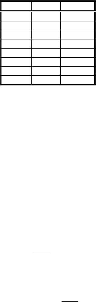
Figure 1.1: (a) Rectangle with sides x and y. Area is A = xy. I hope you knew tha t. (b) Rectangula r box
with sides x, y and z. Volume is V = xyz. I hope you knew that too.
If we have to convert 3.68 ×10
4
s to minutes, we would use a conversion factor with seconds
in the denominator (to cancel what we’ve got alre ady; the conversion factor is still equal to
1). So:
3.68 × 10
4
s = (3.68 × 10
4
s)
1 min
60 s
= 613 mi n
1.1 .3 Math: You Had This In High School. Oh, Yes You Did.
The mathematical demands of a “non–calculus” physics course are not extensive, but you
do have to be proficient with the little bit of mathematics that we will use! It’s just the stuff
you had in high school. Oh, yes you did. Don’t tell me you didn’t.
We will often use scientific notation to express our numbers, because this allows us
to express large and small numbers conveniently (and also express the precision of those
numbers). We will need the basic algebra operations of powers and roots and we will solve
equations to find the “unknowns”.
Usually the algebra will be very si mple. But if we are ever faced with an equation that
lo oks like
ax
2
+ bx + c = 0 (1.1)
where x is the unknown and a, b and c are given numbers ( constants) then there are two
possible answers for x which you can find from the quadratic formula:
x =
−b ±
√
b
2
− 4ac
2a
(1.2)
On occasion you will need to know some facts from geometry. Starting simple and working
upwards, the simplest shapes are the rectangle and rectangular box, shown in Fig. 1.1. I f
4 CHAPTER 1. MATHEMATICAL CON CEPTS
R
R
(a)
(b)
D
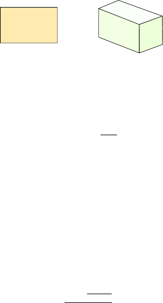
Figure 1.2: (a) Circle; C = πD = 2π R; A = πR
2
. (b) Sphere; A = 4πR
2
; V =
4
3
πR
3
. You’ve seen these
formulae before. Oh, yes you have.
R
h
h
A
(a)
(b)
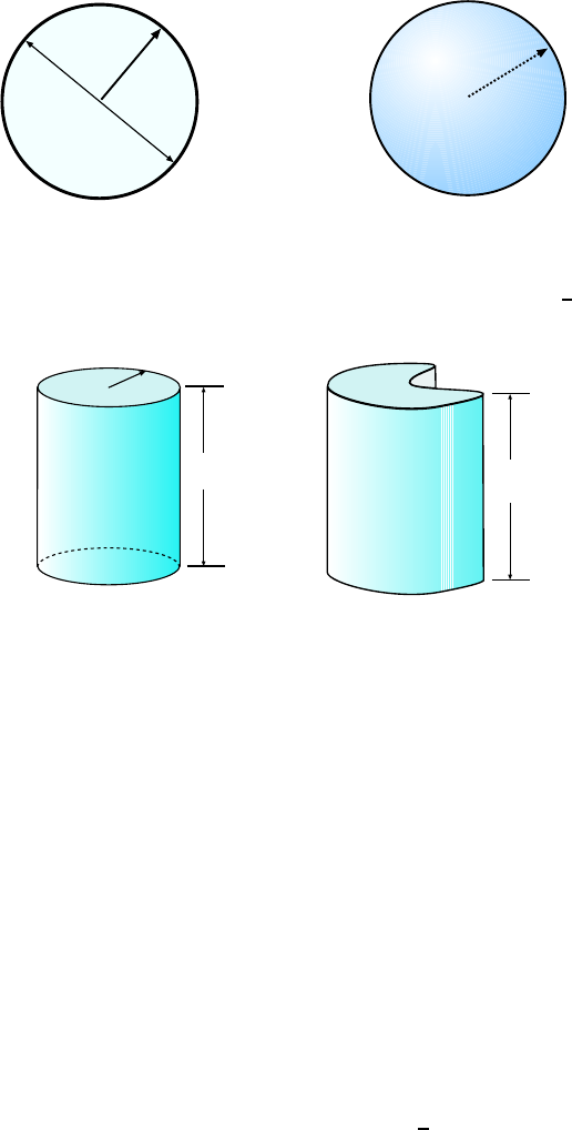
Figure 1.3: (a) Circular cylinder of radius R and height h. Volume is V = πR
2
h. (b) Right cylinder of
arbitrary shape. If the area of the cross section is A, the volume is V = Ah.
the rectangle has sides x and y its area is A = xy. Since it is the product of two lengths,
the units of area in the SI system are m
2
. For the rectangular box with sides x, y and z, the
volume is V = xyz. A volume is the product of three lengths so its units are m
3
.
Other formulae worth mentioning her e are for the circle and the sphere; see Fig. 1.2.
A circle is specified by its radius R (or its diameter D, which is twice the radius). The
distance around the circle is the circumference, C. The circumfe r ence and area A of the
circle are given by
C = πD = 2πR A = πR
2
(1.3)
A sphere is specified by its r adius R. The surface area A and volume V of a sphere are
given by
A = 4πR
2
V =
4
3
πR
3
(1.4)
Another simple shape is the (right) circular cylinder, shown in Fig. 1.3(a). If the c ylinder
has radius R and height h, its volume is V = πR
2
h. This is a special case of the general
right cylinder (see Fig. 1.3(b)) where if the area of the cross section is A and the height is
h, the volume is V = Ah.
1.1. THE IMPORTANT STUFF 5
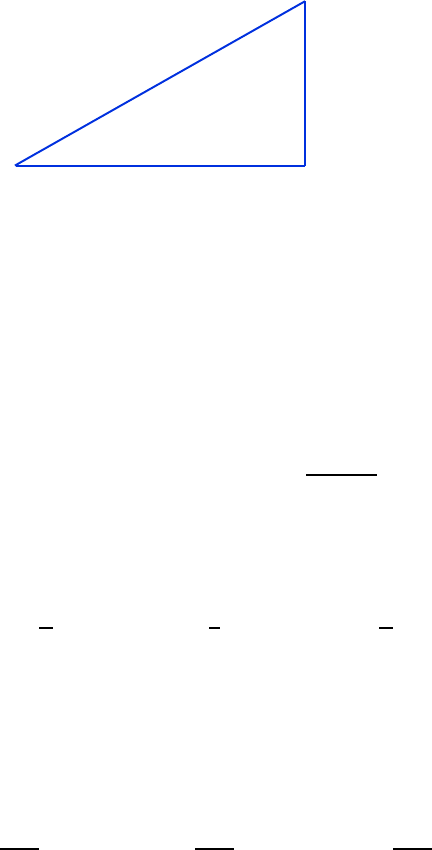
a
b
c
q
f
Figure 1.4: Right triangle with sides a, b and c.
1.1 .4 Math: Trigonometry
You will also nee d some simple t r igonometry. This won’t amount t o much more than relating
the side s of a right triangle, that is, a triangle with two sides joined at 90
◦
.
Such a triangle is shown in Fig. 1.4. The sides a, b and c are related by the Pyt hagorean
Theorem:
a
2
+ b
2
= c
2
=⇒ c =
√
a
2
+ b
2
(1.5)
We only need the angle θ to determ ine the shape of the triangle and this gi ves the ratios
of the sides of t he triangle. The ratios are given by:
sin θ =
a
c
cos θ =
b
c
tan θ =
a
b
(1.6)
Or you can remember these ratios in term of their positions with respect to the angle θ. If
the side s are
a = opposite b = adjacent c = hypothenuse
then the ratios are
sin θ =
opp
hyp
cos θ =
adj
hyp
tan θ =
opp
adj
(1.7)
If you pick out the first letters of the “words” in Eq. 1.7 in order, they spell out SOHCAH-
TOA. If you want to remember the trig ratios by intoning “SOHCAHT OA”, be my guest,
but don’t do it near me.
1.1 .5 Vectors and Vector A ddition
Throughout our study of physics we will discuss quantities which have a size (that is, a
magnitude) as well as a direction These quantities are called vectors. Examples of vectors
are velocity, acceleration, force, and the electric field.
6 CHAPTER 1. MATHEMATICAL CON CEPTS
A
B
C
A
B
Figure 1.5: Vectors A and B are added to give the vector C = A + B.
A
x
A
y
A
y
x
Figure 1.6: Vector A is split up into components.
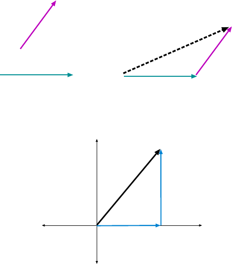
Vectors are represented by arrows which show their magnitude and direction. The laws
of physics will req uire us to add vectors, and to represent this operation on paper, we add
the arrows. The way t o add arrows, say to add arrow A to arrow B we join the tail of B to
the head of A and then draw a new arrow from the tail of A to the head of B. The result
is A + B. This is shown in Figure 1.5.
Vectors can be multiplied by ordinary numbers (called scalars), giving new vectors, as
shown in Fig. 1.5.
1.1 .6 Components of Vectors
Addition of vectors would be rather messy if we didn’t have an easy technique for handling
the trigonometry. Vector addition is made much easier when we split the vectors into parts
that run along the x axis and parts that run along the y axis. These are called the x and y
components of the vector.
In Figure 1.6A vector split up into components: One component is a vector that runs
along the x axis; the other is one running along the y axis.
If we let A be the magnitude of vector A and θ is its direc tion as measured counter–
1.1. THE IMPORTANT STUFF 7
y
x
y
x
A
A
(a)
(b)
Figure 1.7: Vectors can have negative components when they’re in the other quadrants.
clockwise from the +x axis, then the component of this vector that runs along x has length
A
x
, where the relation between the two is:
A
x
= A cos θ (1.8)
Likewise, the length of the component that runs along y is
A
y
= A sin θ (1.9)
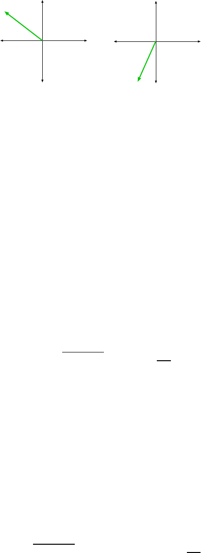
Actually, we don’t literally mean “length” here since that implies a positive number.
When t he vector A has a direction lying in quadrants II, III or IV (as in Figure 1.7, then
one of its components will be negative. For example, if the vector’s direction is in quadrant
II as in Fig. 1. 7(a), its x component is negative while its y component is positive.
Now if we have the components of a vector we can find its magnitude and direction by
the following relations:
A =
q
A
2
x
+ A
2
y
tan θ =
A
y
A
x
(1.10)
where θ is the angle which gives the direction of A, measured counterclockwise from the +x
axis.
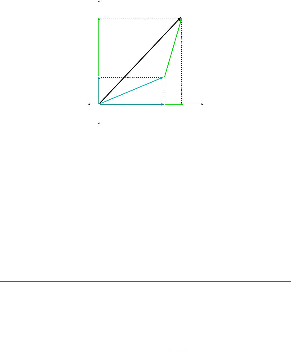
Once we have the x and y components of two vectors it is easy to add the vectors since
the x components of the individual vectors add to give the x component of the sum, and
the y comp onents of the individual vectors add to give the y component of the sum. This is
illustrated in Figure 1.8. Expressing this with math, if we say that A + B = C, we mean
A
x
+ B
x
= C
x
and A
y
+ B
y
= C
y
(1.11)
One we have the x and y components of the total vector C, we can get the m agnitude
and direction of C with
C =
q
C
2
x
+ C
2
y
and tan θ
C
=
C
y
C
x
8 CHAPTER 1. MATHEMATICAL CON CEPTS
C
A
B
A
x
B
y
A
y
B
x
x
y
Figure 1.8: Vectors A and B add to gi ve the vector C. The x components o f A and B add to give the x
component of C: A
x
+ B
x
= C
x
. Likewise for the y components.
Summing up, many problems involving vectors will give you the m agnitudes and direc-
tions of two vectors and ask you to find the magnitude and direction of their sum. To do
this,
• Find the x and y components of the two vectors.
• Add the x and y parts individually to get the x and y parts of the sum (resultant vector).
• Use Eq. 1.10 (trig) to get the magnitude and direction of the resultant.
1.2 Worked Examples
1.2 .1 Measurement and Units
1. The mass of the parasitic wasp Caraphractus cintus can be as smal l as 5×10
−6
kg.
What is this mass in (a) grams (g), (b) milligrams (mg) and (c) micrograms (µg)?
[CJ6 1-1]
(a) Using the fact that a kilogram is a thousand grams: 1 kg = 10
3
g, we find
m = 5 × 10
−6
kg = (5 × 10
−6
kg)
10
3
g
1 kg
!
= 5 × 10
−3
g
1.2. WORKED EXAMPLES 9
(b) Using the fact that a milligram is a thousandth of a gram: 1 mg = 10
−3
g, and our
answe r from (a), we find
m = 5 ×10
−3
g = (5 × 10
−3
g)
1 mg
10
−3
g
!
= 5 mg
(c) Using the fact that a microgram is 10
−6
(one millionth) of a gram: 1 µg = 10
−6
g
m = 5 ×10
−3
g = (5 × 10
−3
g)
1 µg
10
−6
g
!
= 5 × 10
3
µg
2. Vesna Vulovic survived the longest fall on record wit hout a parachute when
her pl ane exploded and she fell 6 miles, 551 yards. What is the distance in meters?
[CJ6 1-2]
Convert the two lengths (i. e. 6 miles and 551 yards) to meters and then find the sum.
Use the fact that 1 mil e equals 1.6093 km to get:
6 mile = (6 mile)
1.6093 km
1 mile
!
10
3
m
1 km
!
= 9656.1 m
and we can use the exact relation 1 in = 2.54 cm to get
551 yd = (551 y d)
36 in
1 yd
!
2.54 cm
1 in
1 m
10
2
cm
= 503.8 m
Add the two lengths:
L
Total
= 9656.1 m + 503.8 m = 1.0160 × 10
4
m
3. How many seconds are there in (a) one hour and thirty–five minutes and (b)
one day? [CJ6 1-3]
(a) Change one hour to seconds using the unit–factor method:
1 h = (1 h)
60 min
1 h
60 s
1 min
= 3600 s
10 CHAPTER 1. MATHEMATICAL CON CEPTS
Likewise change 35 min to seconds:
35 min = (35 min)
60 s
1 min
= 2100 s
The total is
1 h + 35 min = 3600 s + 2100s = 5700 s
(b) Change one day to seconds; use the unit factors:
1 day = (1 day)
24 h
1 day
!
60 min
1 h
60 s
1 min
= 86, 400 s
4. Bicyclists in the Tour de France reach speeds of 34.0 miles per hour (mi/h) on
flat sections of the road. What is this speed in (a) kilometers per hour (km/h)
and (b) meters per second (m/s)? [CJ6 1-4]
(a) Use the relation between miles and kilometers:
1 mi = 1.609 km
to get
v = 34.0
mi
h
= (34.0
mi
h
)
1.609 km
1 mi
!
= 54.7
km
h
(b) U sing our answer from ( a) along with the r elations
1 km = 10
3
m and 1 hr = (60 min)
60 s
1 min
= 3600 s
to get
v = (54.7
km
h
)
1 h
3600 s
!
10
3
m
1 km
!
= 15.2
m
s
1.2 .2 Trigonometry
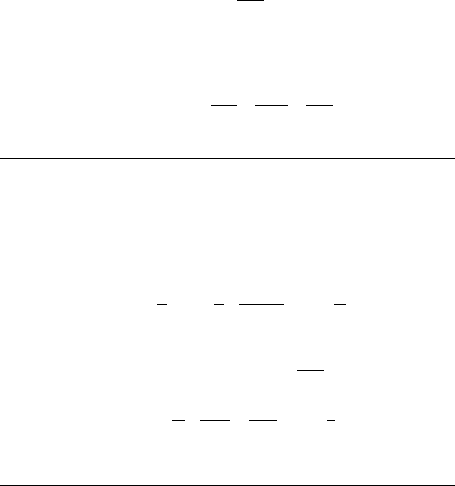
5. For the right t riangle with sides as shown in Figure 1.9, find side x and the
angle θ.
1.2. WORKED EXAMPLES 11
6.20
3.50
x
q
Figure 1.9: Right triangle for example 5.
7.10
y
x
36
o
Figure 1.10: Right triangle for example 6.
We can use the Pythagorean theorem to find x . Pythagoras tells us:
x
2
+ (3.50)
2
= (6.20)
2
Solving for x gives
x
2
= (6.20)
2
−(3.50)
2
= 26.19 =⇒ x =
√
26.19 = 5.12
As for θ, since we are given the “opposite” side and the hypothenuse, we know sin θ. It
is:
sin θ =
3.50
6.20
= 0.565
Then get θ with the inverse sine operation:
θ = sin
−1
(0.565) = 34.4
◦
6. For the right triangle with the side and angle as shown in Figure 1.10, find
the missing sides x and y.
We don’t know the “opposite” side y but we do know the angle to which it is opposite.
So we can write a relation involving the sine of the angle, thus:
sin 36
◦
=
y
7.10
=⇒ y = (7.10) sin 36
◦
= 4.17
12 CHAPTER 1. MATHEMATICAL CON CEPTS
45
o
2.60
1.50
q
45
o
2.60
1.50
q
y
(a)
(b)
Figure 1.11: Right triangle for example 7.
Likewise, we can wri t e a relation involving the “adjacent” side and the cosine of the
angle,
cos 36
◦
=
x
7.10
=⇒ x = ( 7.10) cos 36
◦
= 5.74
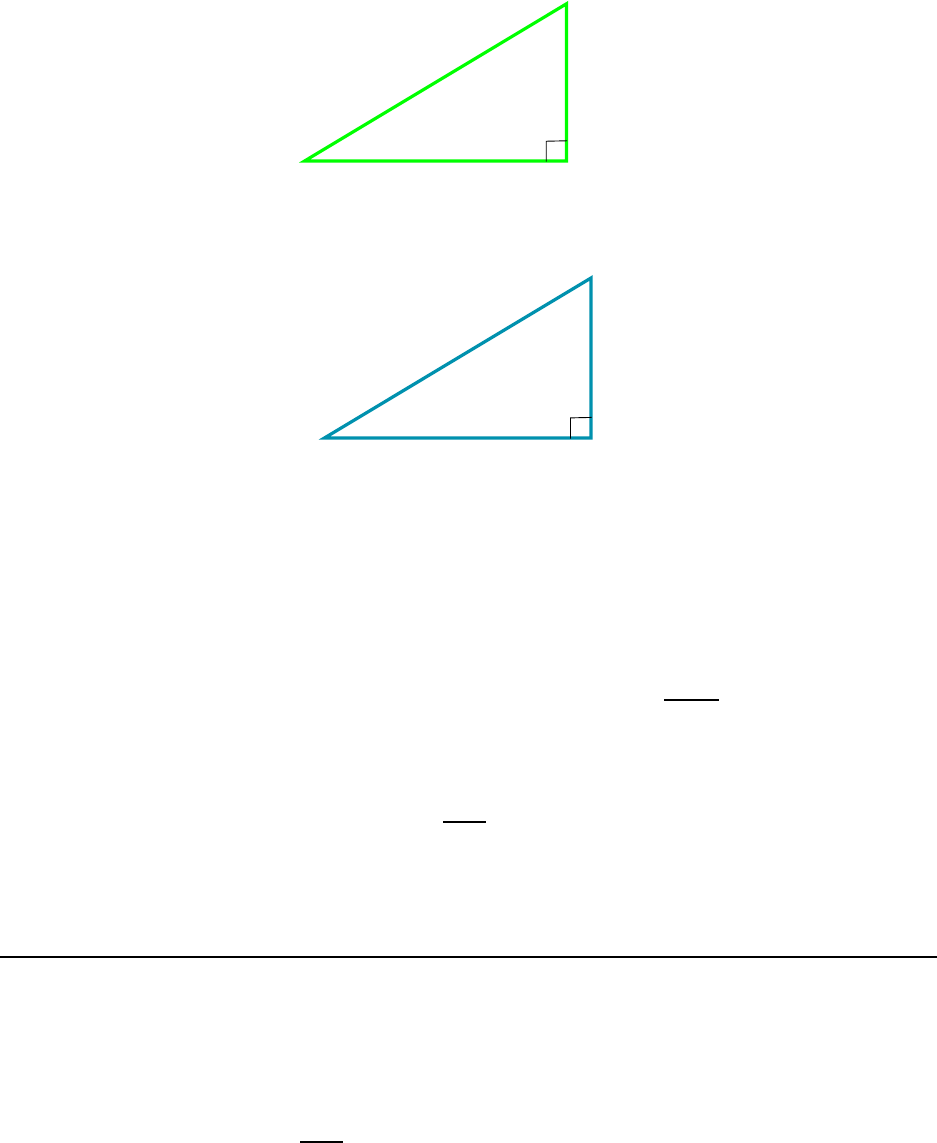
7. Find the missing angle θ in Figure 1.11(a). (The right angles in the figure are
marked.)
It wi ll help to first find the length of the side marked y in Fig. 1.11(b). Since y and the
side of length 2.60 are the opposite and adjacent sides of the 45
◦
angle, we have:
tan 45
◦
=
y
(2.60)
=⇒ y = (2.60) tan 45
◦
= 2.60
We can write a similar relation for the missing angle,
tan θ =
y
(1.50)
=
2.60
1.50
= 1.73
Using the inverse tangent operation,
θ = tan
−1
(1.73) = 60.0
◦
The missing angle is 60.0
◦
.
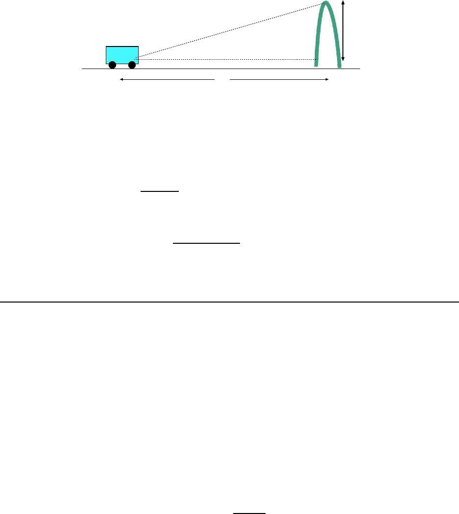
8. You are driving into St. Louis, Mi ssouri and in the distance you see the
famous Gateway–to–the–West arch. This monument rises to a height of 192 m.
You esti mate your line of sight with the top of the arch to be 2.0
◦
above the
horizontal. Approximately how far (in kilometers) are you from the base of the
arch? [CJ6 1-11]
1.2. WORKED EXAMPLES 13
2.0
o
x
192 m
Figure 1.12: Gateway Arch is viewed from car.
The situation is diagrammed in Figure 1.12. (Of course the ground is not exactly flat and
your eyeballs are not quite at ground level but these details don’t make much difference.)
If the distance of the car from the base of the arch is x then we have
(192 m)
x
= tan(2.0
◦
) = 3.49 × 10
−2
Solve for x:
x =
(192 m)
(3.49 × 10
−2
)
= 5.50 × 10
3
m
= 5.50 km
The car is about 5.50 km from the base of the arch.
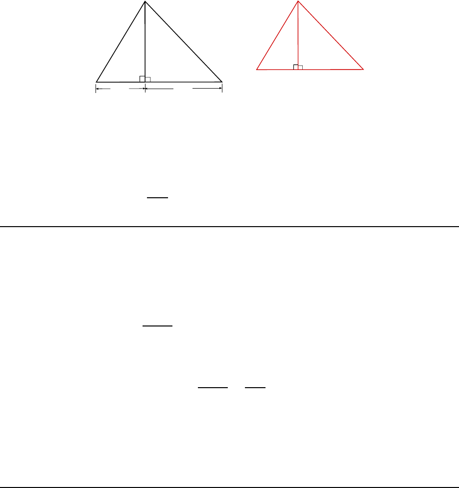
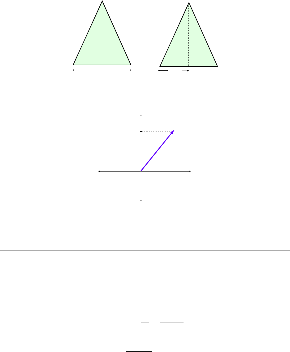
9. The silhouette of a Christmas tree is an isosceles tri angle. The angle at the
top of the triangle is 30.0
◦
, and the base measures 2.00 m across. How t all is the
tree? [CJ6 1-15]
The triangle described in the problem is shown in Fig. 1.13(a). By “isoscel es” we mean
that the two angles at the bottom are the same and as a result the two sides have the same
length.
We can drop a line from the top of the triangle to the base; this line divides the base into
two equal parts, and since the l ength of the whole base is 2.0 m, the length of each part is
1.0 m. This is shown is Fig. 1.13(b). Let the height of the triangle be calle d y.
Now si nce the angles in a triangle must all add up to 180
◦
we have
2θ + 30
◦
= 180
◦
=⇒ 2θ = 150
◦
=⇒ θ = 75
◦
and the n we can write
tan θ =
y
1.00 m
and the n solve for y:
y = (1.00 m) tan θ = (1.00 m) tan 75
◦
= 3.73 m
14 CHAPTER 1. MATHEMATICAL CON CEPTS
30
o
2.0 m
q
q
y
(a)
(b)
1.0 m
Figure 1.13: Isoceles–triangle shaped Christmas tree
52
o
y
x
290 N
Figure 1.14: Force vector for Example 10.
1.2 .3 Vectors and Vector A ddition
10. A force vector points at an angle of 52
◦
above the +x axis. It has a y
component of +290 newtons. Find (a) the magnitude and (b) the x compone nt of
the force vector. [CJ6 1-38]
(a) The vector (which we’ll call F) is shown in Fig. 1.14. We know F
y
and the direction of
F. With F standing for the magnitude of F , we have
sin(52
◦
) =
F
y
F
=
(290 N)
F
Then solve for F :
F =
(290 F)
(sin 52
◦
)
= 368 N
1.2. WORKED EXAMPLES 15
5.0 m
2.1 m
0.5 m
y (N)
x (E)
R
20
o
Figure 1.15: Displacements of the golf ball in Example 11.
(b) We also have
tan(52
◦
) =
F
y
F
x
=
(290 N)
F
x
Then solve for F
x
:
F
x
=
(290 N)
(tan 52
◦
)
= 227 N
11. A golfer, putting on a green, requires three strokes to “hole the ball”. During
the first putt, the ball rolls 5.0 m due east. For the second putt, the ball travels
2.1 m at an angle of 20.0
◦
north of east. The third putt is 0.50 m due north. What
displacem ent (magnitude and direction relative to due east) would have been
needed to “hole the ball” on the very first putt? [CJ6 1-41]
The directions and magnitudes of the individual putts are shown in Fig. 1.15. The vectors
are joined head–to–tail , showing the total displacement of the ball. The total displacement
(which we call R) is also shown.
Note, the first vector only has an x component. The last vector only has a y component.
We add up the xcomponents of t he three vectors:
R
x
= 5.0 m + (2.1 m) cos 20
◦
+ 0.0 m = 6.97 m
And we add up the y components of the three vectors:
R
y
= 0.0 m + (2.1 m) sin 20
◦
+ 0.50 m = 1.22 m
The magnitude of the net displacement is
R =
q
R
2
x
+ R
2
y
=
q
(6.97 m)
2
+ (1.22 m)
2
= 7.1 m
16 CHAPTER 1. MATHEMATICAL CON CEPTS
B
A
C
60.0
o
20.0
o
+x
+y
Figure 1.16: Vectors for Example 12.
and the dir ection of the net displacement, as measured in the usual way (“North of East”)
is given by θ, where
tan θ =
R
y
R
x
=
(1.22)
(6.97)
= 0.175
so that
θ = tan
−1
(0.175) = 9.9
◦
Had the golfer hit the ball giving it this magnitude and direction, the ball would have
gone in the hole with one hit, which is calle d a double–Bogart or something to that effect.
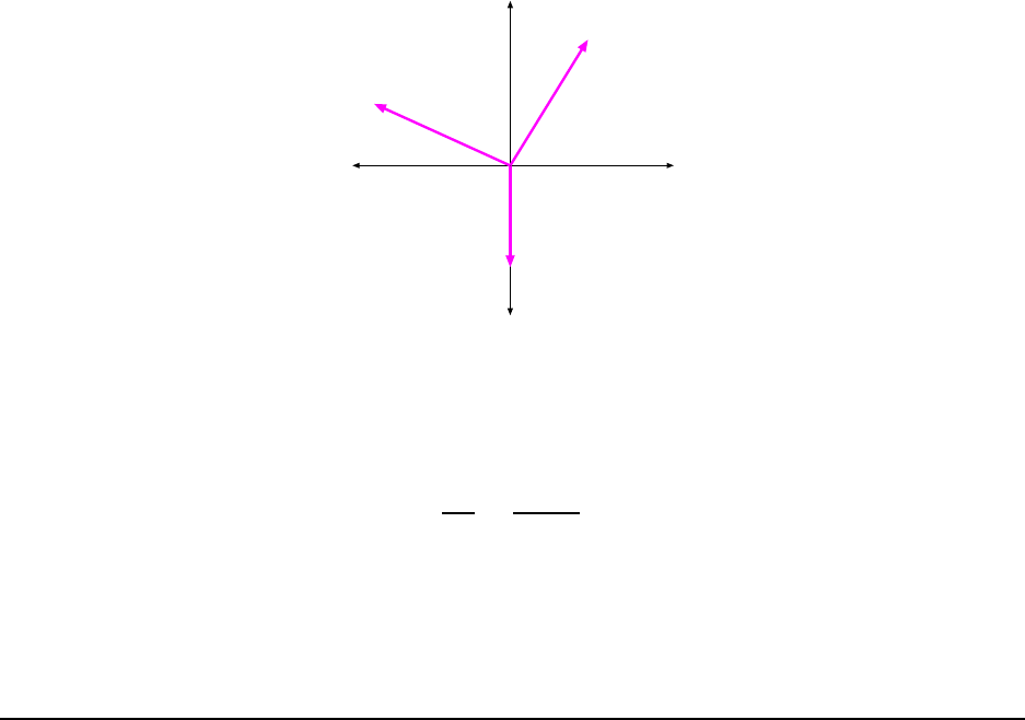
12. Find the resultant of the three displacement vectors in Fig. 1.16by means of
the component method. The magnitudes of the vectors are A = 5.00 m, B = 5.00 m
and C = 4.00 m. [CJ6 1-43]
First find the individual components of each of the vectors. Note, the angles given in the
figure are measured in different ways so we have to think about the signs of the c omponents.
Here, the x component of vector A is negative and the y component of vector C (which is
all it’s got!) is also negative.
Using a li t tle trig, the components of the vectors are:
A
x
= −(5.00 m) cos(20.0
◦
) = −4.698 m
A
y
= +( 5.00 m) sin(20.0
◦
) = +1.710 m
B
x
= +( 5.00 m) cos(60.0
◦
) = +2.500 m
B
y
= +( 5.00 m) sin(60.0
◦
) = +4.330 m
1.2. WORKED EXAMPLES 17
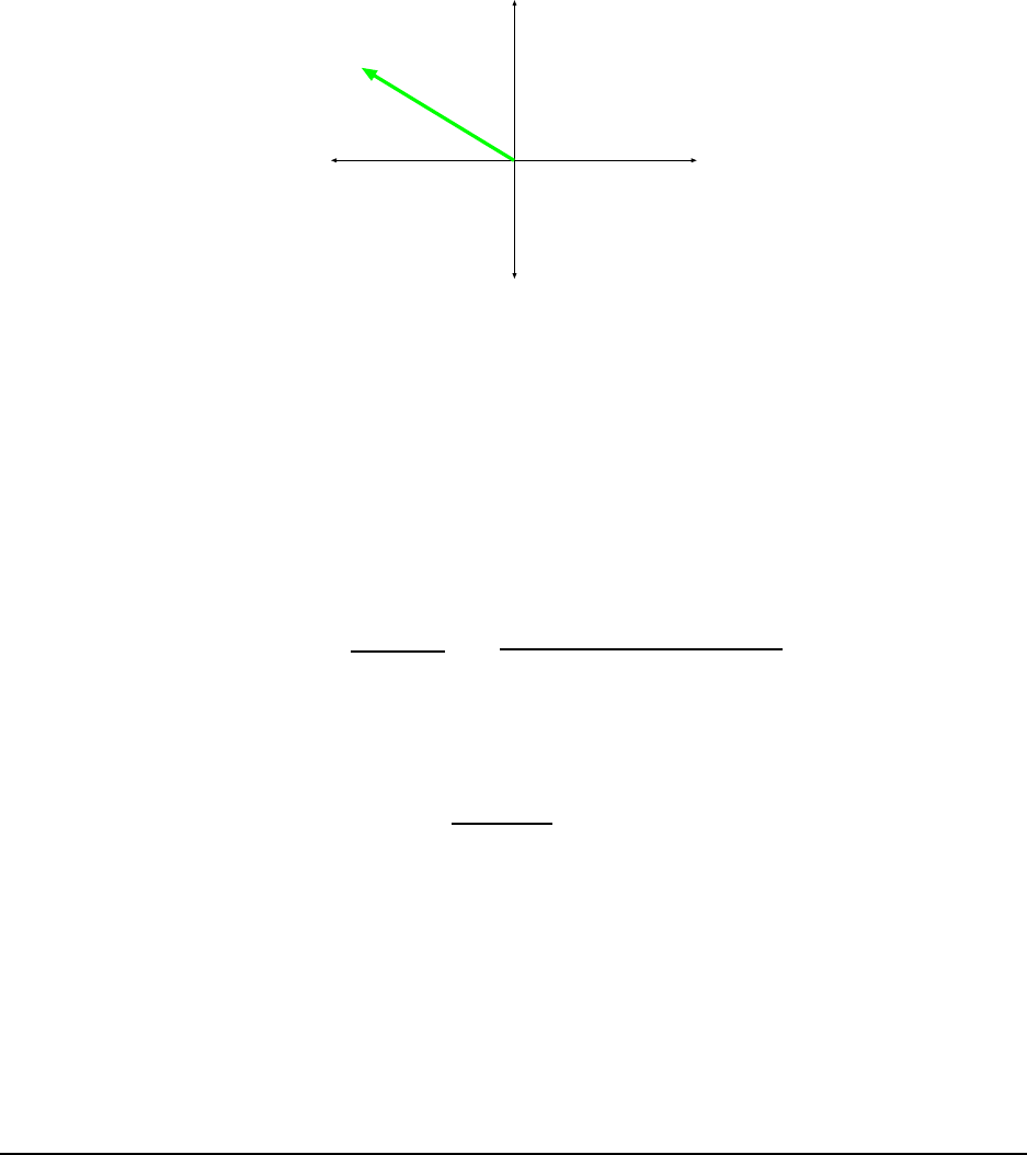
R
y
x
Figure 1.17: Vector R lies in quadrant II.
and
C
x
= 0 C
y
= −4.00 m
The resultant (sum) of all three vectors (which we call R) then has components
R
x
= A
x
+ B
x
+ C
x
= −4.698 m + 2.500 m + 0 m = −2.198 m
R
y
= A
y
+ B
y
+ C
y
= + 1.710 m + 4.330 m − 4.000 m = 2.040 m
This gives the co mponents of R. The magnitude of R is
R =
q
R
2
x
+ R
2
y
=
q
(−2.198 m)
2
+ (2.040 m)
2
= 3.00 m
If the direction of R (as measured from the +x axis) is θ, then
tan θ =
2.040
(−2.198)
= −0.928
and naively pushing the tan
−1
key on the calculator would have you believe that θ = −42.9
◦
.
Such vector would lie in the “fourth quadrant” as we usually call it. But we have found that
the x component of R is negative while the y comp onent is positive and such a vector must
lie in the “second quadrant”, as shown in Fig. 1.17. What has happened is that the calculator
returns an angle that is wrong by 180
◦
so we need to add 180
◦
to the naive angle to get the
correct angle. So the direction of R is really given by
θ = −42.9
◦
+ 180
◦
= 137.1
◦
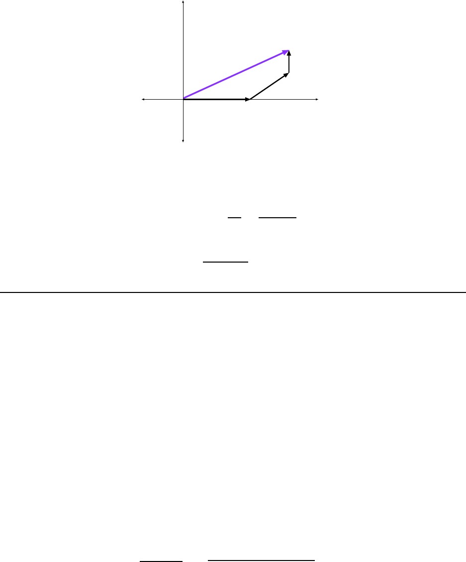
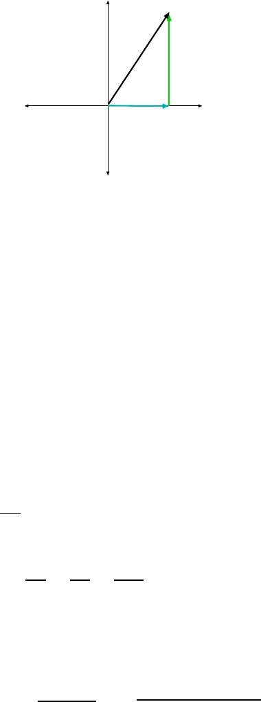
13. Vector A has a magnitude of 6.00 units and points due east. Vector B points
due north. (a) What is the magnitude of B, if the vector A+ B points 60.0
◦
north
of east? (b) Find the magnitude of A + B. [CJ6 1-47]
18 CHAPTER 1. MATHEMATICAL CON CEPTS
A
B
A+B
60
o
x
y
6.00
Figure 1.18: Vectors A and B for example 13.
(a) Vectors A and B are shown in Fig. 1.18. The components of A are
A
x
= 6.00 A
y
= 0
and we also know that B
x
= 0, but we don’t know B
y
. But if the sum of A and B is R:
R = A + B
Then the components of R are given by
R
x
= A
x
+ B + x = 6.00 + 0.00 = 6.00 R
y
= A
y
+ B
y
= 0 + B
y
= B
y
But we are given the direction of R, namely θ = 60.0
◦
, so that
R
y
R
x
= tan θ = tan(60.0
◦
) = 1.732
But then this tells us:
R
y
R
x
=
B
y
A
x
=
B
y
6.00
= 1.732
Solve for B
y
:
B
y
= (6.00)(1.732) = 10.32
(b) The magnitude of A + B (that is. R ) is
R =
q
R
2
x
+ R
2
y
=
q
(6.00)
2
+ (10.32)
2
= 11.94
Chapter 2
Motion in One Dimension
2.1 The Important Stuff
2.1 .1 Displacement
We begin with moti on that takes place along a straight line, for example a c ar speeding
up along a straight road or a rock which is thrown straight up into the air. The concepts
introduced here will be useful when we solve harder problems with motion in two dimensions.
We often talk about the motion of a “particle”. This just means that the object in
question i s small in siz e c ompared to the distance that it moves for the times of interest, so
that we don’t need to worry about its actual siz e or orientation.
We map out the possible positions of the particle with a coordinate (system) which
might be labelled x (or y). Changes in position are given by changes in the value of x; we
write a change in x as ∆x.
The change in coordinate ∆x is the displacement that the particle undergoes; it will
occur over some time interval ∆t. Displacements have units of length (meters) and can be
positive or negative!
If we divi de the displacement by the time interval we get the average velocity for the
particle for the given time period ∆t.
2.1 .2 Speed a nd Velocity
When an obje ct undergoes a displacement ∆x in a time interval ∆t, the ratio is the average
velocity v for that time interval:
v =
∆x
∆t
(2.1)
Velocity has units of length divided by time; in physics, we will usuall y express velocity
in
m
s
.
19
20 CHAPTER 2. MOTION IN ONE DIMENSION
The average velocity de pends on the time interval chosen for the measurement ∆x and
as such isn’t a very useful quantity as far as physics is concerned. A more useful idea is that
of a velocity associated with a given moment in time. This is found by calculating v for a
very small time interval ∆t which includes the time t at which we want this velocity.
The instantaneous velocity v is given by:
v =
∆x
∆t
for “very small” ∆t. (2.2)
The instantaneous velocity has a definite value at each point in time.
The idea of an instantaneous velocity is familiar from the fact that you can tell the speed
of a car at a given time by looking at its spe edometer. Your speedometer might tell you
that you are travelling at 65
mi
hr
. That doesn’t mean that you intend to drive 65 mi or that
you intend to drive for 1 hour! It means what Eq. 2.2 says: At the time you looked at
the speedometer, a small displacement of the car divided by the corresponding small time
interval gives 65
mi
hr
. (Of c ourse, when we use the idea in physics, we use the metric system!
We wi ll us
m
s
.)
The concept of taking a ratio of terms which are “very small” is central to the kind of
mathematics k nown as calculus. Even though this course is supposed to be “non–calculus”
we have to cheat a little because the idea of instantaneous velocity is so important!!
2.1 .3 Motion With Constant Velocity
When an object starts off at the origin (so that x = 0 at time t = 0) and its velocity is
constant, then
x = v
0
t Constant velocity!! (2.3)
Which is the familiar equation often stated as “distance equals speed times time”. It is only
true when the velocity of the object is constant. But in physics the really interesting c ases
are when the velocity is not constant.
2.1 .4 Accel eration
We need one more idea about motion to do physics. The (instantaneous) velocity of an
object can change. I t can change slowly (as when a car gradually gets up to a cruising
speed) or it can change rapidly (as when you re al ly hit the gas pedal or the brakes in your
car). The rate at which velocity changes is important in physics.
If the velocity of an object undergoes a change ∆v over a time period ∆t we define the
average accele ration over that period as:
a =
∆v
∆t
(2.4)
2.1. THE IMPORTANT STUFF 21
Acc eleration has units of
m
s
divi ded by seconds (s) which we write as
m
s
2
.
As wit h velocity, the average quantity is not as important as the “right–now” quantity so
we need the idea of an instantaneous acceleration. Therefore at any given time want to know
that rati o of ∆v to ∆t f or a very small change in time. The instantaneous acceleration
a is given by:
a =
∆v
∆t
for “very small” ∆t. (2.5)
Generally the acceleration of an object can change with time. Now, since it’s a free
country we could ask how rapidly the acceleration is changing, but it turns out that this
is not so imp ortant for physics. Furthermore for a great many of our problem s the moving
object will have a constant acceleration.
2.1 .5 Motion Where the Ac celeration is Consta nt
As we will see later on, the case of constant acceleration is e ncountered often because this is
what happens when there is a constant force acting on the object. In the following equations
we assume that we’re talking about a particle whose acceleration a is constant.
If the object accelerates uniformly (i.e. it moves wi t h constant a) then its velocity changes
by the same amount for equal changes in the time t. We can express this as:
a =
∆v
∆t
We will now introduce some notation that will be used in the next couple chapters: We
will say that when we discuss the m otion of a particle over a certain time period, the clock
starts at t = 0. So if we ask about the velocity and position at a l ater time, that later time
is just called “t”. We will say that the velocity of the particle at t = 0 is v
0
, and its velocity
at the time t is v. Then we have ∆v = v − v
0
and ∆t = t, and t he last equation can b e
rewritten as:
v = v
0
+ at (2.6)
Next , we ask about the displacement of the particle at time t, given that it started off
with a velocity v
0
. Recal l that we had a formula for x in Eq. 2.3 but when there is an
acceleration that equation is no longer true!!! (In fact it is no longer meaningful since it is
not clear what “v” means.)
Again we will say that the particle is initially located at x = 0, that is, it is initially at
the origin. Then the displacement of the particle at time t is given by:
x = v
0
t +
1
2
at
2
(2.7)
By combining these equations we can show:
v
2
= v
2
0
+ 2ax (2.8)

22 CHAPTER 2. MOTION IN ONE DIMENSION
which can be useful because i t does not contain the time t. We can also show:
x =
1
2
(v
0
+ v)t (2.9)
which can be useful b ecause it does not contain the accele r ation a. But in order to use this
equation we must know beforehand that the acceleration is constant.
2.1 .6 Free -Fall
The most common kind of acceleration which we encounter in daily life is the one which an
object undergoes when we drop it or throw it up in the air. Before stating the value of this
acceleration we need to be clear about the coordinates used to descri be the motion of an
object in (one–dimensional) free–fall.
In our free–fall problems we will always have the y axis point straight up regardless of
the ini t ial motion of the object. So when y increases the object is moving upward and the
velocity v wi ll be positive; when y de creases the obj ect is moving downward and the velocity
v will b e negative
It turns out —for reasons we can understand only after learning about forces— that when
an object is moving vertically in free–fall its velocity decreases by 9.80
m
s
every second. This
is true when the object is moving upward and when it is moving downward and for that
matter when the object has reached its maximum height. Then the rate of change of the
object’s velocity has a constant value given by
a =
∆v
∆t
=
(−9.80
m
s
)
(1 s)
= −9.80
m
s
2
The minus sign is important and comes from the fact that our y axis points upward but
things fall downward. This number is known as the acceleration of gravity.
Before going to o far we should say that the acce leration of falling objects has this value
over the surface of the Earth and that the value may be slightly different depending on
lo cation, i.e. at some place on earth the value may be more like −9.81
m
s
2
.
The magnitude of acceleration of gravity is such an important number in physics that we
give it the name, g, so that to a good approximation we can use
g = 9.80
m
s
2
(2.10)
But be careful : g is defined as a posi tive number, and with our y axis going upward, the
value of a (the acceleration for a freely-falling objec t ) is a = −g. Signs are i mportant!
2.2. WORKED EXAMPLES 23
v
0
= 69 m/s
v
= 6.1 m/s
750 m
Figure 2.1: Jet landing and decreasing its speed, in Example 1.
2.2 Worked Examples
2.2 .1 Motion Where the Ac celeration is Consta nt
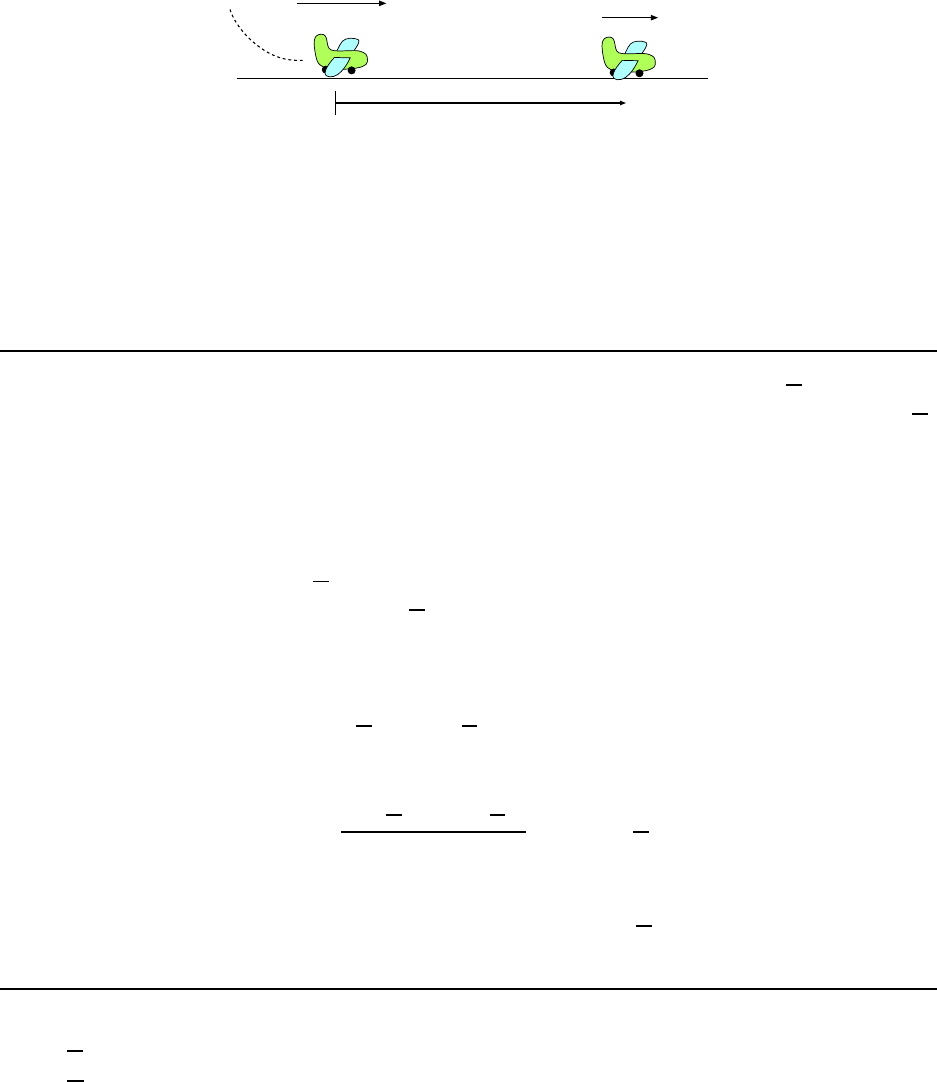
1. A jetliner, travelling northward, is landing with a speed of 69
m
s
. Once the
jet touches down, it has 750 m of runway in which to reduce its speed to 6.1
m
s
.
Compute the average acceleration (magnit ude and direction) of the plane during
landing. [CJ6 2-25]
We organize ourselves by drawi ng a picture of the landing plane, as shown in Fig. 2.1.
The plane touches down at x = 0; that’s where the motion begins, as far as we’re concerned.
The initial velocity is v
0
= 69
m
s
. In the final position (after it has travelled the full extent
of the runway), x = 750 m and v = 6.1
m
s
. B ut we are not given the time t for this motion
to t ake placed and we don’t know t he (constant) accele r ation a.
If we want to get a we can use Eq. 2.8, because it doesn’t cont ai n the time t. Plugging
in the numbers, we get:
(6.1
m
s
)
2
= (69
m
s
)
2
+ 2a(750 m)
Do some algebra and solve for a:
a =
(6.1
m
s
)
2
− (69
m
s
)
2
2(750 m)
= −3.15
m
s
2
We get a negative answer, and we expect that; the plane’s velocity (in the direction of motion,
North) is decreasing. The acceleration has a magnitude of 3.15
m
s
2
and its direction is opposite
the direction of moti on, i.e. South.
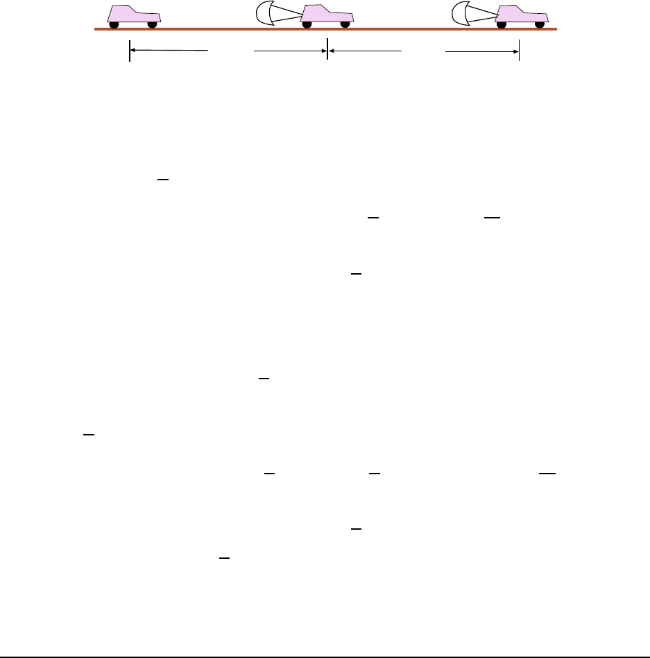
2. A drag racer, starting from rest, speeds up for 402 m with an acceleration of
+17.0
m
s
2
. A parachute t hen opens, slowing the car down wit h an acceleration of
−6.10
m
s
2
. How fast is the racer moving 3.50 ×10
2
m after the parachute opens? [CJ6
2-28]
24 CHAPTER 2. MOTION IN ONE DIMENSION
402 m
350 m
a = 17.0 m/s
2
a = - 6.10 m/s
2
Figure 2.2: Mo tion of the drag racer i n Example 2.
A diagram of the motion wil l help! This is shown in Fig. 2.2. First, let’s find the velo city
of the racer at the time the chute opened. We can use Eq. 2.8; with v
0
= 0 (the racer starts
from rest), a = +17.0
m
s
2
and x = 402 m, solve for v:
v
2
= v
2
0
+ 2ax = 2(402 m)(17
m
s
2
) = 6.83 ×10
3 m
2
s
2
So then
v = 82.7
m
s
Now consider the part of the motion after the chute opens; we must consider it separately
since the acceleration here is different from the first part of the motion. For this part of the
motion the initial velocity is the value we found for the final veloc ity of the earlier motion:
v
0
= 82.7
m
s
Second part of motion
We have the distance covered for this part of the motion (x = 350 m ) and the acceleration
(a = −6.10
m
s
2
; the racer’s velocity decreases during this part) and we can again use Eq. 2.8:
v
2
= v
2
0
+ 2ax = (82.7
m
s
)
2
+ 2(−6.10
m
s
2
)(350 m) = 2.56 × 10
3
m
2
s
2
and this gives
v = 50.6
m
s
The racer has a speed of 50.6
m
s
when it has moved 350 m past the point where the chute
opene d.
2.2 .2 Free -Fall
3. A penny is dropped from the top of the Sears Tower in Chicago. Considering
that the height of the buil ding is 427 m and ignoring air resistance, find the speed
with which the penny strikes the ground. [CJ6 2-37]
A picture of the problem is given in Fig. 2.3, where we’ve drawn the coordinate axi s. The
2.2. WORKED EXAMPLES 25
y
0
y = -427 m
a = -9.8 m/s
2
Sears
Figure 2.3: Penny dropped from top of Sears Tower in Example 3.
penny begins its motion at y = 0 and since it falls down, its coordinate upon striking the
ground is −427 m. Since we dro p the penny its initial velocity is v
0
= 0 and its acceleration
during the fall is a = −g = −9. 8
m
s
2
.
We are looking for the final velocity v but we don’t have the time of the fall. We can use
Eq. 2.8 since that equation doesn’t contain t. We find:
v
2
= v
2
0
+ 2ax
= 0
2
+ 2(−9.8
m
s
2
)(−427 m)
= 8.37 × 10
3
m
2
s
2
Taking the square root of this number gives 91.5
m
s
but there are really two answers for v,
namely ±91.5
m
s
, and since the penny is falling downward when it hit the ground we want
the negative one:
v = −91.5
m
s
.
But the answer to the que stion is that the penny’s speed (the absolute value of v) was 91.5
m
s
when it hit the ground.
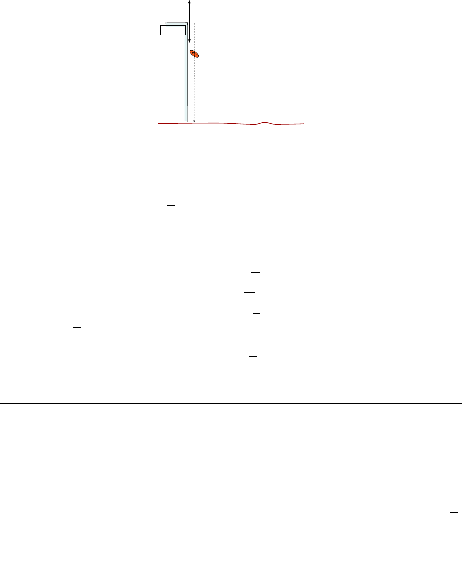
4. From her bedroom window a girl drops a water–filled balloon to the ground,
6.0 m below. If the balloon is released from rest, how long is it in the air? [CJ6
2-41]
The problem is diagrammed in Fig. 2. 4. The coordinate system is shown; the positive y
axis poi nts up, and (as always) we assume that the ball oon starts its motion at y = 0. But
if that is the case, then when the balloon hits the ground, its y coordinate is −6.0 m.
The init ial velocity of the balloon is v
0
= 0 and its acceleration is a = −g = −9.80
m
s
2
.
To find how long the balloon i s in the air, we ask the question: At what tim e is y equal to
−6.0 m? We c an then find t using Eq. 2.7. So we write:
−6.0 m = 0 +
1
2
(−9.80
m
s
2
)t
2
26 CHAPTER 2. MOTION IN ONE DIMENSION
6.0 m
v
0 = 0
Figure 2.4: Water–balloon is dropped in Example 4.
t = 2.00 s
v
0
Figure 2.5: Rock is tossed up in the air in Example 5.
and solve for t. We find:
t
2
=
2(−6.0 m)
(−9.80
m
s
2
)
= 1.22 s
2
and the n
t = 1.11 s
The balloon hits the ground at t = 1.11 s, so it spends 1.11 s in the air.
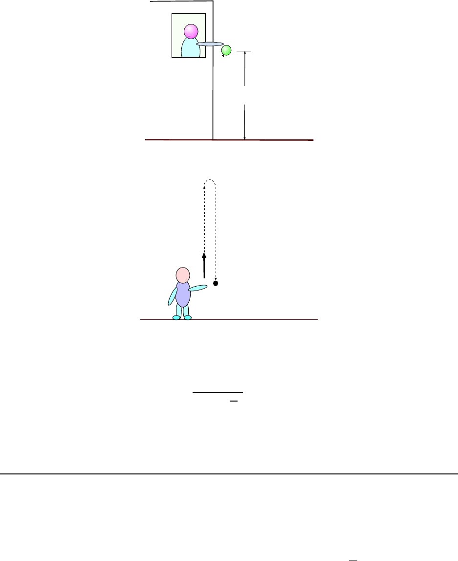
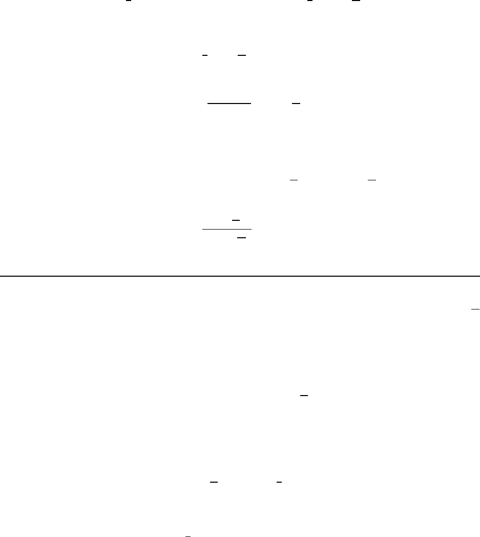
5. A bal l thrown verticall y upward is caught by the t hrower after 2.00 s. Find
(a) the initial speed of the ball and (b) the maximum height the ball reaches.
[Ser7 2-48]
(a) We sketch t he problem in Fig. 2.5. The ball has some initial spee d v
0
(which we don’t
know). We know the acceleration of the ball, name ly a = −g = −9.80
m
s
2
. We also know that
2.2. WORKED EXAMPLES 27
at t = 2.00 s the y coordinate of the ball was zero. (As usual, we say the ball starts off at
y = 0.) If we put that information into Eq 2.7 we get:
x = v
0
t +
1
2
at
2
=⇒ 0 = v
0
(2.00 s) +
1
2
(−9.80
m
s
2
)(2.00 s)
2
and now we can solve this for v
0
:
v
0
(2.00 s) =
1
2
(9.80
m
s
2
)(2.00 s)
2
= 19.6 m
This gives:
v
0
=
(19.6 m)
(2.00 s)
= 9.80
m
s
(b) We know that at maximum height the veloc ity v is zero. We can use Eq 2.8 to get
the value of y at this time:
v
2
= v
2
0
+ 2ay =⇒ 0 = (9.80
m
s
)
2
+ 2(−9.80
m
s
2
)y
Solve this for y and get:
y =
(9.80
m
s
)
2
2(9.80
m
s
2
)
= 4.90 m
so the maximum height attained by the ball was 4.90 m.
6. An astronaut on a distant planet wants to determine its acceleration due
to gravity. The astronaut throws a rock straight up with a velocity of +15
m
s
and measures a time of 20.0 s before the rock returns to his hand. What is the
acceleration (magnitude and direction) due to gravity on this planet? [CJ6 2-39]
A diagram of the path of the r ock is shown in Fig. 2.6. The y axis is measured upward
from the position of the hand.
We know the initial velocity of the ro ck, v
0
= +15.0
m
s
but we don’t know the value of
the acce leration, a
y
. (We do know that it will be a negative number , because objects fall
down on this planet too!) We know that at t = 0.0 s y is 0.0 m (of course) but we also know
that at t = 20.0 s, y is equal to 0.0 s.
If we put the second piece of information into Eq. 2.7 we get
0.0 = (15.0
m
s
)(20.0 s) +
1
2
a(20.0 s)
2
from which we can find a. Some algebra gives us:
1
2
a(20.0 s)
2
= −300 m
28 CHAPTER 2. MOTION IN ONE DIMENSION
v
0
= 15 m/s
t = 20.0 s
Figure 2.6: Path of tossed rock in Example 6.
12 m/s
110 m
Figure 2.7: Ma n throws rock downward wi th speed 12
m
s
, in Example 7.
Then:
a = −
2(300 m)
(20.0 s)
2
= −1.50
m
s
2
The magnitude of the acc eleration due to gravity on the planet is 1.50
m
s
2
and from the minus
sign we know that the direction of the acceleration is downward. (No surprise... things fall
down on other planets as well!
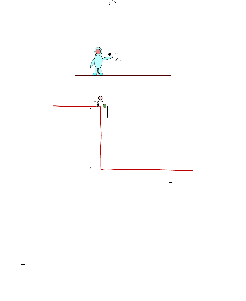
7. A man st ands at the edge of a cliff and throws a rock downward with a speed
of 12.0
m
s
. Sometime later it strikes the ground 110 m below the place where it
was thrown. (a) How long does it take to reach t he ground? (b) What is the
speed of the rock at impact?
(a) The problem is illustrated in Fig. 2.7. Since the rock is thrown downward, the initial
velocity of the rock is v
0
= −12.0
m
s
, and of course a = −9.80
m
s
2
. When the rock hit s the
2.2. WORKED EXAMPLES 29
ground its y coordinate is y = −110 m, so in this part we are asking “At what time does
y = −110 m?”
y is given by
y = v
0
t +
1
2
at
2
= (−12.0
m
s
)t −
1
2
(9.80
m
s
2
)t
2
so we just need to solve
−110 m = (−12.0
m
s
)t −
1
2
(9.80
m
s
2
)t
2
Dropping the units for simplicity, a little algebra gives
(4.90)t
2
+ (12.0)t − 110 = 0
which is a quadratic equation. (Recall Eq. 1.1.) Using the quadratic formula, there are two
possible answers, given by
t =
(−12.0) ±
q
(12.0)
2
+ 4(4.90)(110)
2(4.90)
.
A little calculator work gives the two (?) answers:
t = −6.12 s or t = 3.67 s
So which is the answer? (There can only be one time of impact!) The answer must be the
second one because a negative time t is meaningless; the rock was thrown at t = 0. Therefore
the rock takes 3.67 s to reach the ground.
(b) We need to find the velocity of the rock at the the time found in part (a). The velocity
of the rock is given by
v = v
0
+ at = (−12
m
s
) + (−9.80
m
s
2
)t
so at t = 3.67 s it is
v = (−12.0
m
s
) − (9.80
m
s
2
)(3.67 s) = −18.1
m
s
and so the speed of the rock at impact is 18.1
m
s
.
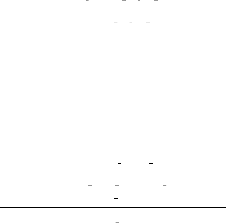
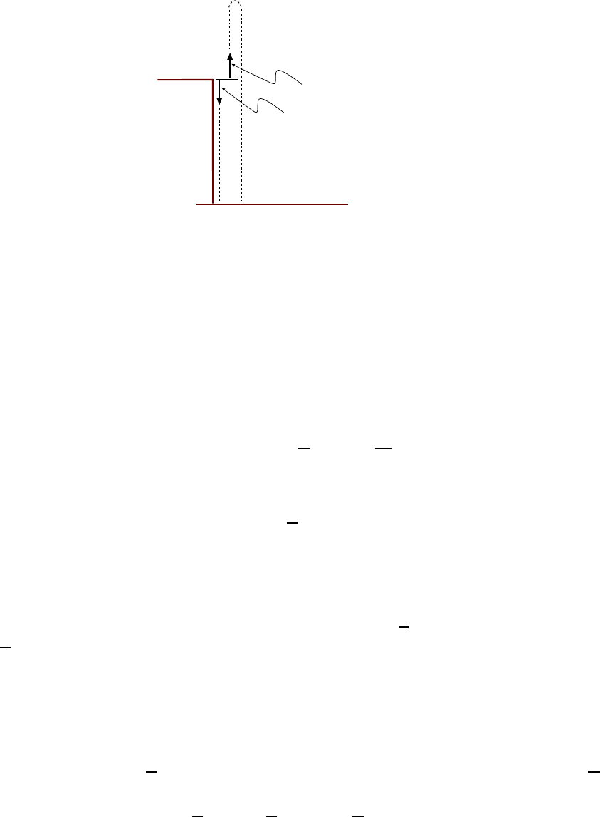
8. Two ide ntical pellet guns are fired simultaneously from the edge of a cliff.
These guns impart as initial speed of 30.0
m
s
to each pellet. Gun A is fired str aight
upward, with the pellet going up and falling back down, eventually hitti ng t he
ground beneath the cliff. Gun B is fired straight downward. In the absence of air
resistance, how long after pellet B hits the ground does pellet A hit the ground?
[CJ6 2-43]
30 CHAPTER 2. MOTION IN ONE DIMENSION
v
0
= -30.0 m/s
v
0
= +30.0 m/s
Figure 2.8: Two pellet guns shoot pellets; pellet from Gun A goes up then down. Pellet from B goes
straight down.
Ho o! This one sounds complicated. And they didn’t even tell us how high the cl iff is!
(Doesn’t it matter?) We draw a picture of the problem, as in Fig. 2.8.
It turns out that if we understand something about the motion of pell et A the problem
is much simpl er. Let’s ask: What is the velocity v of pel let A when it returns to the height
at which it was thrown? Here we don’t care about the time, just the distances and velocities
are involved, so we want to use Eq. 2.8. When the pellet returns to the original height then
y = 0 and so we get:
v
2
= v
2
0
+ 0 = (+30
m
s
)
2
= 900
m
2
s
2
and the proper soluti on to this equation is
v = −30
m
s
.
Here we choose the minus sign b ecause the pellet is moving downward at that time. So when
the pellet returns to the same height it has the same speed but is moving in the opposite
direct ion.
But recall that pell et B was thrown downward with speed 30
m
s
, that is, its initial velocity
was −30
m
s
. So fr om this point on, the motion of pellet A is the same as that of pellet B. So
from that point on it will be the same amount of time unt il A hits the ground. Therefore
the amount of time which A spends in the air above that spent by B is the tim e it spends it
takes to go up and then down to the ori gi nal height. Therefore we now want to answer the
question: H ow long does it take A to go up and back to the original height?
To answe r this question we can use Eq. 2.7 with x = 0. We can also ask how long it take
until the velocity eq uals −30
m
s
, and that will be simpler. So using Eq. 2.6 with a = −9.80
m
s
2
we solve for t:
−30
m
s
= + 30
m
s
+ (−9.80
m
s
2
)t
2.2. WORKED EXAMPLES 31
We get:
t =
(−60
m
s
)
(−9.80
m
s
2
)
= 6.1 s
Summing up, it takes 6.1 s for pellet A to go up and back down to the original height;
this is the amount of tim e it spends in the air longer than the tim e B is in the air. So pellet
A hits the ground 6.1 s after B hits the ground.
32 CHAPTER 2. MOTION IN ONE DIMENSION
Chapter 3
Motion in Two Dimensions
3.1 The Important Stuff
3.1 .1 Motion in T wo Dimensions, Coordinates and Displacement
We wi ll now deal with more general motion, motion which does not take place only along a
straight line.
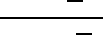
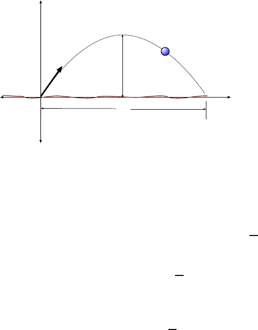
An example of this is shown in Fig. 3.1, where a ball is thrown not straight up, but at
some angle θ from the horizont al . The motion of the ball takes place in a plane and i ts
trajectory (path) through the air happe ns to have the shape of a parabola.
To describe the position of the ball, we now need two coordinates, namely x and y,
defined as shown i n the figure. Here we have chosen to put the origin of the coordinate
system at the place where the ball begins its motion with t he positive y axis pointing “up”,
as in the last chapter. We will usuall y make this choice, although we are free to make other
choices for the placement of the axes... as long as we stick with our choices!
y
x
q
Figure 3.1: Tossed ball and coordinate system to describe its motion.
33
34 CHAPTER 3. MOTION IN TWO DIMENSIONS
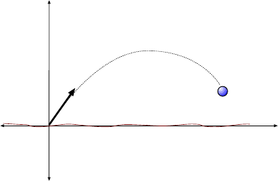
r
1
r
2
Dr
y
x
r
y
x
(a)
(b)
Figure 3.2: (a) Object’s posi tion is given by the displacement vector r. (b) Change in the displacement
vector as the object moves. ∆r ha s components ∆x and ∆y.
The coordinates of the ball, (x and y) are the two components of the displacement
vector, which we will write as r. As the ball moves, the displace ment vector changes. In
Fig. 3.2(b) we show a change in location for an object. The displacement vector changes
from r
1
to r
2
, resulting in the change ∆r = r
2
−r
1
. The components of ∆r are ∆x and ∆y.
3.1 .2 Velocity and Acceleration
Whereas in the previous chapter we only had one coordinate changing with time, now we
have two: x and y. In a time interval ∆t both co ordinates will change.
We can now study the ratio of ∆x to ∆t and the ratio of ∆y to ∆t. These ratios are the
average x and y velocities for the interval ∆t:
v
x
=
∆x
∆t
v
y
=
∆y
∆t
(3.1)
As before, the really interesting quantity, as far as physics is concerned, is (are) the
instantaneous x and y velocities. These are the velocities we compute when the time interval
is extremely small. . . as sm all as we can imagine:
v
x
=
∆x
∆t
for small ∆t v
y
=
∆y
∆t
for small ∆t (3.2)
These eq uations define the x and y velocitie s v
x
and v
y
at a particular point in time. These
velocities can change with time, and the rate of change of these velociti es are the accelera-
tions: The x and y accelerations, respectively.
v
x
and v
y
are t he x− and y− components of the velocity ve ctor. The magnitude of t he
velocity vector,
v =
q
v
2
x
+ v
2
y
(3.3)
3.1. THE IMPORTANT STUFF 35
is called the (instantaneous) speed of the particle. Speed is always a positive number and
like velocity it has units of
m
s
.
The instantaneous x and y accelerations are defined by:
a
x
=
∆v
x
∆t
for small ∆t a
y
=
∆v
y
∆t
for small ∆t (3.4)
and a
x
and a
y
are the x− and y− components of the acceleration vector.
Basically the equations given above don’t involve any new it ideas from those given in
the last chapter. What is new is the fact that we are finding t hese quantiti es (velocity and
acceleration) for the x and y coordinates separately, and in our problem solving we will have
to thi nk about both coordinates at once, so the problems will generally be more challenging.
3.1 .3 Motion When the Acceleration Is Constant
Though one can study all kinds of two–dimensional motion at this point, we will have
enough trouble on our hands if we just settle for the simple case when both of the acceleration
components are constant. In that case, both components of the velocity will change uniformly
with tim e. Suppose at ti me t = 0 the velocity components v
x
and v
y
have the values v
0x
and
v
0y
. (These are the initial values of the velocity components.) Then the values of v
x
and
v
y
later on will be given by
v
x
= v
0x
+ a
x
t v
y
= v
0y
+ a
y
t (3.5)
These equations have the same form but they are re ally different equations because in general
a
x
and a
y
will have different values in a physics problem; v
0x
and v
0y
will also be different.
If we want to find the value of the coordinates x and y at time t (assuming the particle
starts from the origin, x = 0 and y = 0 at time t = 0) then we can use:
x = v
0x
t +
1
2
a
x
t
2
y = v
0y
t +
1
2
a
y
t
2
(3.6)
Again, these equations look ali ke but they pertain to the two parts of a particle’s motion:
The horizontal (x) part and the vertical (y) part.
Just as in the one-dimensional case we have an equation relating v, a and x but not
containing the time t:
v
2
x
= v
2
0x
+ 2a
x
x v
2
y
= v
2
0y
+ 2a
y
y (3.7)
36 CHAPTER 3. MOTION IN TWO DIMENSIONS
y
x
q
0
v
0
R
H
Figure 3.3: A special projectile problem; projectile is fired at angle θ
0
and initial speed v
0
.
3.1 .4 Free Fall; Projectile Problems
When an object is moving freely (e. g. it has been thrown or is dropped) near the surface of
the earth, it undergoes a downward acceleration of magnitude g = 9.80
m
s
2
. This means that
if our y axis points upward then
a
x
= 0 and a
y
= −9.80
m
s
2
= −g
The horizontal acceleration here is zero... things don’t fall sideways! But the vertical accel-
eration is −g. . . things do fall down!
Again, the symbol g in these notes stands for +9.80
m
s
2
.
Since the horizontal acceleration is zero, the x component of the velocity stays the same
all through the motion, i.e. v
x
= v
0x
during the flight of the projectile.
3.1 .5 Ground–To–Ground Proje c tile: A Long Example
In this section we solve a special case for a projectile , the case where the projectile b egins
and ends its motion at the same height. We will get some results which are interesting and
can be used in some problems, but one must keep in mind that if we have a projectile whose
initial and final heights are not t he same, these results are not relevant!
The deri vation given here i nvolves more math than usual for these notes, but again, the
result is interesting enough that it is worth it.
We consider the motion of a projectile fired from ground level, as shown in Fig. 3.3, at
angle θ
0
upward from the horizontal and a speed v
0
. The projectile goes up and comes back
down, striking the ground at the s ame level at which it was fired. We are interested in
finding how long the projectile was in fli ght, t he horizontal distance it travels (called the
range, R) and its maximum height H. We are treating v
0
and θ
0
as if that are already
known so that R and H will be expressed in terms of these values.

3.1. THE IMPORTANT STUFF 37
From the magnitude and direction of the initial velocity vector v
0
we get the components
of the initial velocity:
v
0x
= v
0
cos θ
0
v
0y
= v
0
sin θ
0
We will first answer the question: How long is the proje ctile in fli ght? That is the same as
asking: “At what time do es y equal zero”? Since a
y
= −g, the y part of Eq. 3.6 gives
y = 0 = (v
0
sin θ
0
)t −
1
2
gt
2
for which we can factor the right hand side to get
0 = t
v
0
sin θ
0
−
gt
2
There are two solutions to this equation. These are:
t = 0 or
gt
2
= v
0
sin θ
0
⇒ t =
2v
0
sin θ
0
g
The first of these possibilit ies is a correct answer to the question but not the one we want!
The second solution gives us the time of impact:
t =
2v
0
sin θ
0
g
(3.8)
To find the range R we ask: “What is the value of x at the time of impact?”. Use the
result in Eq. 3.8 and the x part of Eq. 3.6 (r emembe r ing that a
x
= 0 for a projectile!):
x = (v
0
cos θ
0
)t −
1
2
a
x
t
2
(3.9)
= (v
0
cos θ
0
)
2v
0
sin θ
0
g
!
− 0 (3.10)
=
2v
2
0
sin θ
0
cos θ
0
g
(3.11)
This answer can be made a lit tle simpler using a formula from trigonometry,
sin 2θ
0
= 2 sin θ
0
cos θ
0
so our result is
R =
2v
2
0
sin θ
0
cos θ
0
g
=
v
2
0
sin 2θ
0
g
(3.12)
Two interesting features of this solution can be noted:
38 CHAPTER 3. MOTION IN TWO DIMENSIONS
• If we have a definite speed v
0
with which to launch the projectile, to give it the greatest
range we would choose a launch angle of θ
0
= 45
◦
. This is because 45
◦
makes the factor
sin θ
0
the greatest.
• For a given launch speed, if we launch the projectile at either one of a pair of complementary
angles the r ange R will be the same. (For example, θ
0
= 30
◦
and θ
0
= 60
◦
will give the same
range R.) This is because for complementary angles, sin 2θ
0
is the same.
Now we’l l find the maximum height of the projectile. The projectile reaches maximum
height when its y− velocity is zer o (it is i nstantaneously moving neither upward nor down-
ward at that point) so the y part of Eq . 3.5 gives:
v
y
= 0 = (v
0
sin θ
0
) − gt ⇒ t =
v
0
sin θ
0
g
which, you’ll note, is half the total time spent in flight. Thus the project takes as much time
to go up as it does to come down.
The maximum height is the value of y at this time. Using the y part of Eq. 3.6, with
a
y
= −g, we find:
y = v
0y
t +
1
2
a
y
t
2
= (v
0
sin θ
0
)
v
0
sin θ
0
g
!
−
1
2
g
v
0
sin θ
0
g
!
2
=
v
2
0
sin
2
θ
0
g
−
v
2
0
sin
2
θ
0
2g
=
v
2
0
sin
2
θ
0
2g
So the maximum height attained by the projectile is
H =
v
2
0
sin
2
θ
0
2g
(3.13)
Finally we can find the shape of the ball’ s trajectory; we can find this by relating x and
y for the motion of the ball and looking at the relation that we find. Our equations for x
and y were:
x = (v
0
cos θ
0
)t and y = (v
0
sin θ
0
)t −
1
2
gt
2
(3.14)
The first of these gives
t =
x
v
0
cos θ
0
.
Substitute this into the second of the equations in 3.14 and do some algebra; we get:
y = (v
0
sin θ
0
)
x
v
0
cos θ
0
−
1
2
g
x
v
0
cos θ
0
2
= (tan θ
0
)x −
g
2v
2
0
cos
2
θ
0
!
x
2
(3.15)
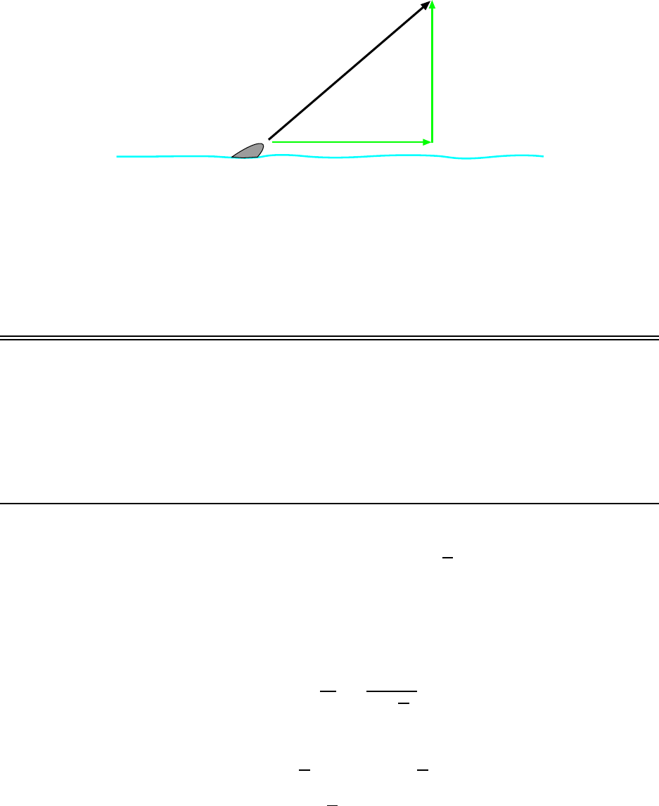
3.2. WORKED EXAMPLES 39
7.7 m/s
v
y
35
o
Figure 3.4: Velocity vector for jumping dolphin in Exampl e 1.
Now while the result in Eq. 3.15 may look like a mess, the important thing to see is that
there i s a y on one side of the equation and an x
2
and x on the other side of the eq uation.
From your usual college algebra class we know that this relation maps out a parabola. In
general the trajectory of a ball tossed through the air is a parabola.
3.2 Worked Examples
3.2 .1 Velocity and Acceleration
1. A dolphin leaps out of the water at an angle of 35
◦
above the horizontal. The
horizontal component of the dolphin’s velocity is 7.7
m
s
. Find the magnitude of
the vertical component of the velocity. [CJ6 3-7]
The velocity vector for the dolphin is drawn in Fig. 3.4. If the vertical component of the
velocity is v
y
, then from trigonometry we know that:
tan 35
◦
=
v
y
v
x
=
v
y
(7.7
m
s
)
And then we can find v
y
:
v
y
= (7.7
m
s
) tan 35
◦
= 5.4
m
s
The vertical component of the velocity is 5.4
m
s
. (That is also its magnitude.
40 CHAPTER 3. MOTION IN TWO DIMENSIONS
3.2 .2 Motion for Co ns tant Acceleratio n
2. On a spacecraft, two engines are turned on for 684 s at a moment when the
velocity of the craft has x and y com ponents of v
0x
= 4370
m
s
and v
0y
= 6280
m
s
.
While the engines are firing, the craft undergoes a displacement that has com-
ponents of x = 4.11 × 10
6
m and y = 6.07 × 10
6
m. Find the x and y components of
the craft’s acceleration. [CJ7 3-12]
For the case of constant acceleration, the displacem ent is related to the initial velocity
and acc eleration by Eq. 3.6. For the x displacement we have
x = v
0x
t +
1
2
a
x
t
2
Plugging in the numbers from the problem, we have
4.11 × 10
6
m = (4370
m
s
)(684 s) +
1
2
a
x
(684 s)
2
From this we can solve for a
x
. We get:
1
2
a
x
(684 s)
2
= 1.12 ×10
6
m =⇒ a
x
=
2(1.12 × 10
6
m)
(684 s)
2
= 4.79
m
s
2
Do the same with the given values for the y displacement. Using
y = v
0y
t +
1
2
a
y
t
2
we have
6.07 × 10
6
m = (6280
m
s
)(684 s) +
1
2
a
y
(684 s)
2
Solve for a
y
:
1
2
a
y
(684 s)
2
= 1.77 ×10
6
m =⇒ a
y
=
2(1.77 × 10
6
m)
(684 s)
2
= 7.59
m
s
2
The acceleration of the craft has components
a
x
= 4.79
m
s
2
and a
y
= 7.59
m
s
2
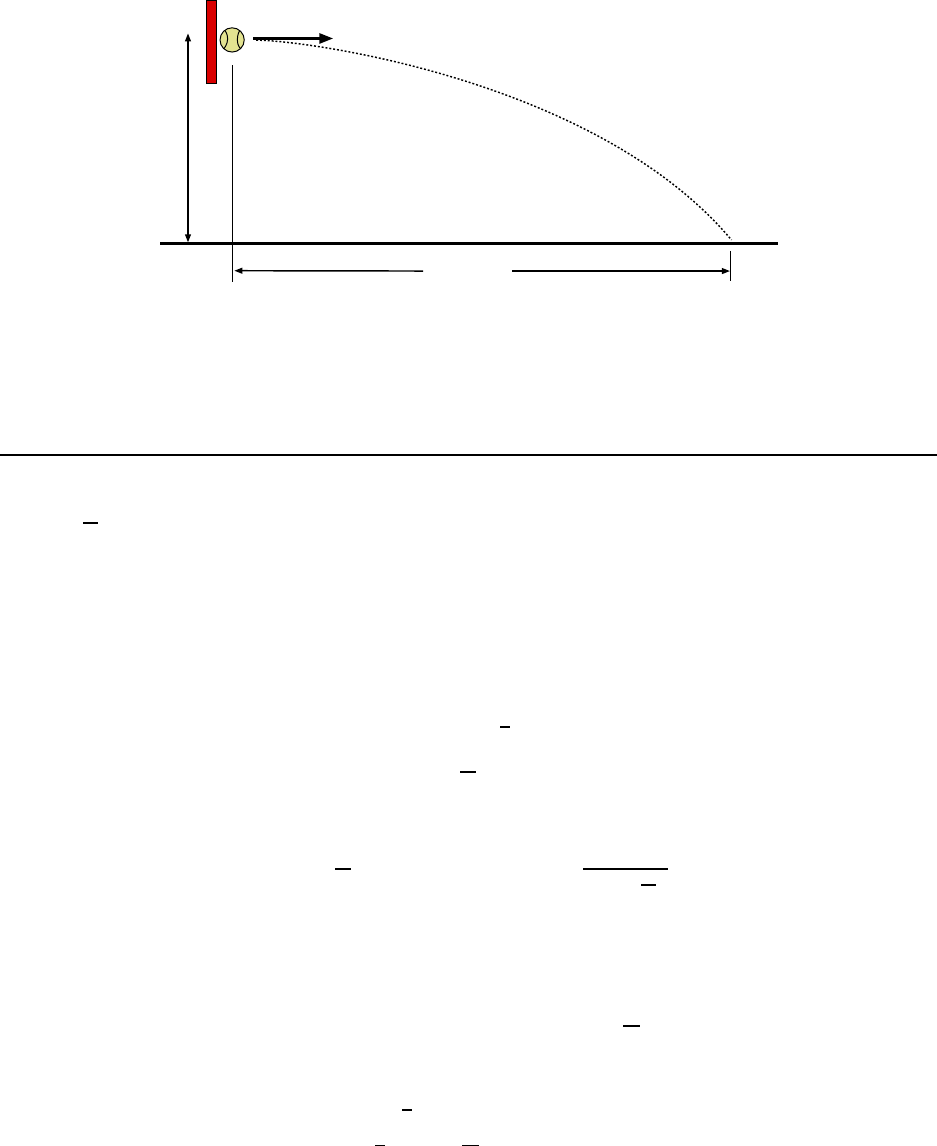
3.2. WORKED EXAMPLES 41
28.0 m/s
19.6 m
?
Figure 3.5: Tennis ball begins its flight horizontally in Example 3.
3.2 .3 Free –Fa ll; Projectile Problems
3. A tennis ball is struck such that it leaves the racket horizontally with a speed
of 28.0
m
s
. The ball hits the court at a horizontal distance of 19.6 m from the
racket. What is the height of the tennis ball when it leaves the racket? [CJ6 3-13]
We draw picture of the ball and it s motion along with the co ordinates, as in Fig. 3. 5.
Let’s first find the time t at which the tennis ball hit the ground. We know t hat when it
hit its x coordinate was equal to 19.6 m. Now from Eq. 3.6, the equation for the x− motion
is
x = v
0x
t +
1
2
a
x
t
2
and here the initial x− velocity is v
0x
= 28.0
m
s
and a
x
= 0 (no sideways acceleration; things
fall d own, not sideways!) The time which gives x = 19.6 m is then found from:
19.6 m = (28.0
m
s
)t + 0 ⇒ t =
(19.6 m)
(28.0
m
s
)
= 0.70 s
Now we can ask: What is the y coordinate of the ball at this time? The answer will give
us the height of the ball when i t was hit.
The ball’s velocity at the beginning of the motion was purely horizontal, so that v
0y
= 0
(no initial y− velocity). The y− accele r ation is a
y
= −9.80
m
s
2
. Then the y part of Eq. 3.6
gives us:
y = v
0y
t +
1
2
a
y
t
2
= 0 +
1
2
(−9.80
m
s
2
)(0.70 s)
2
= −2.4 m
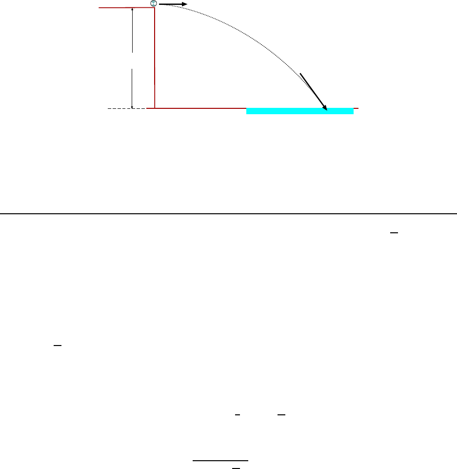
42 CHAPTER 3. MOTION IN TWO DIMENSIONS
11.4 m/s
15.5 m
v
Figure 3.6: Golf ball rolls off a cliff in Example 4.
We get a negative number here because when it hits the ground, the ball has moved downward
from its initial position of y = 0. But to answer the question we say that the initial height
of that ball was 2.4 m.
4. A golf ball rolls off a horizontal cliff with an initial speed of 11.4
m
s
. The ball
falls a vertical distance of 15.5 m into a lake below. (a) How much time does the
ball spend in t he air? (b) What is the speed v of the ball just before it st rikes
the water? [CJ6 3-15]
(a) We draw picture of the ball and its m otion along with the coordinates, as in Fig. 3.6.
Since the y axis goes upward, the l evel of the water is at y = −15.5 m.
Note that the ball rolls off t he cliff horizontally, so that it has an initial x velocity:
v
0x
= 11.4
m
s
, but there is no initial y vel ocity: v
0y
= 0.
To answer (a) we think about the mathematical c ondition that the ball has hit the water.
This is when y = −15.5 m. ( We don’t know the x coordinate of the ball when it hits the
water.) Then using the y part of Eq. 3. 6 with a
y
= −g and v
0y
we can solve for the time t:
−15.5 m = 0 +
1
2
(−9.80
m
s
2
)t
2
So
t
2
=
2(−15.5 m)
(−9.80
m
s
2
)
= 3.2 s
2
and the n
t = 1.8 s
(b) If we have both components of the velocity at the time the ball hits the water, we can
find the speed from Eq. 3.3.
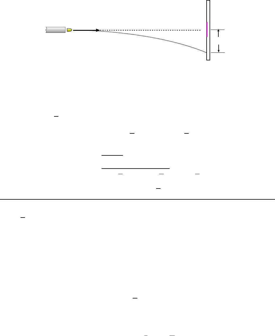
3.2. WORKED EXAMPLES 43
670 m/s
0.025 m
Figure 3.7: Bullet i s fired horizontally at bull’s–eye in Example 5.
Now since there is no x− acceleration, v
x
stays the same as it was at the beginning,
namely v
x
= 11.4
m
s
. Using our answer from (a) and the y part of Eq. 3.6 we find the value
of v
y
at impact:
v
y
= 0 + (−9.80
m
s
2
)(1.8 s) = −17.4
m
s
.
Then the speed of the ball at impact i s
v =
q
v
2
x
+ v
2
y
=
q
(11.4
m
s
)
2
+ (−17.4
m
s
)
2
= 20.8
m
s
The sp eed of the ball when it hits the water is 20.8
m
s
.
5. A horizontal rifle is fired at a bull’s–eye. The muzzle speed of the bullet
is 670
m
s
. The barrel is pointed directly at the center of the bull’s–eye, but the
bullet strikes the target 0.025 m below the center. What is the horizontal distance
between the end of the rifle and the bull’s–eye? [CJ6 3-31]
As usual, begin by drawing a picture of what is happening! The problem is diagrammed
in Fig. 3.7. Even though the rifle is pointed straight at the bull’s–eye, the bullet must miss
because it will take a certain amount of ti me to travel the horizontal distance to the target
and in that time the bullet will have some downward vertical motion.
The rifle was fired horizontally, and from that we know:
v
0x
= 670
m
s
v
0y
= 0
We know that at the time the bullet struck the target its y coordinate was y = −0.025 m.
Then using the y part of Eq. 3.6 we have:
−0.025 m = 0 +
1
2
(−9.80
m
s
2
)t
2
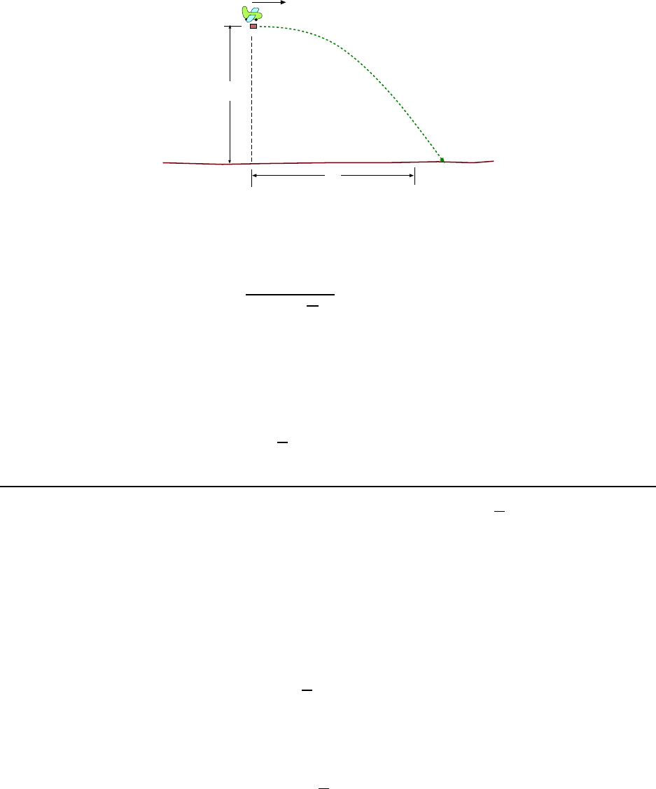
44 CHAPTER 3. MOTION IN TWO DIMENSIONS
R
3100 m
90 m/s
Figure 3.8: Airplane releases a package in Example 6.
which gives us
t
2
=
2(−0.025 m)
(−9.80
m
s
2
)
= 5.1 × 10
−3
t
2
and finally
t = 7.1 ×10
−3
s
The distance to the target is the value of x at the ti me the bullet struck. Now that we
have the t ime of impact we find x using the x part of Eq. 3.6:
x = (670
m
s
)(7.1 × 10
−3
s) = 48 m
6. An airplane is flying horizontally with a speed of 90.0
m
s
at an altitude of
3100 m. The plane releases a package which falls to the level terrain below. At
what distance (measured horizontally from the point of release) doe s the package
strike the ground? Neglect air resistance!
A picture of the problem is given in Fig. 3. 8. The package travels on an arcing path and
eventually hits the ground. Why is this? If the package is “released”, doesn’t it just fall
straight down? No, for reasons that can be bette r appreciated later on, when the package is
“released” it initially has the velo city of its environment, namely that of the plane, and so
the package has an i nitial veloc ity of 90.0
m
s
. After that time though it is in free–fall and its
velocity will change b ecause of the acceleration of gravity. At impact the package has moved
horizontally from its point of release by some distance R.
The package’s initial velocity has only a ho rizontal component, so we have:
v
0x
= 90.0
m
s
v
0y
= 0
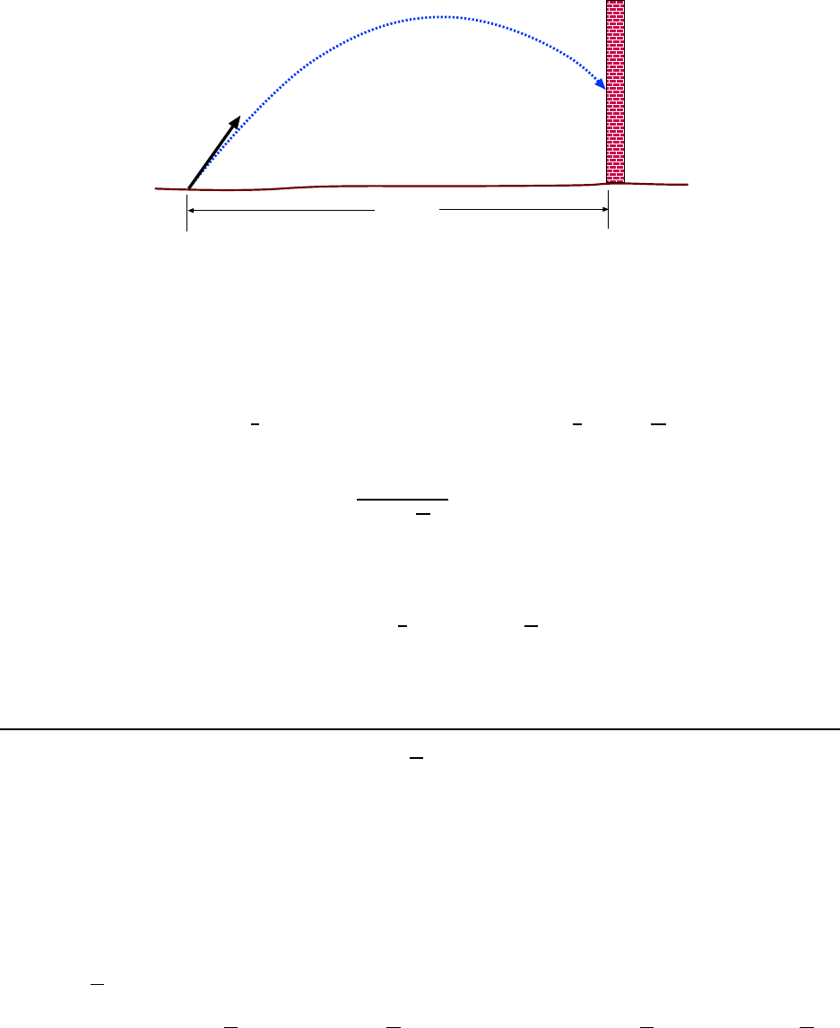
3.2. WORKED EXAMPLES 45
50
o
80 m
35 m/s
Figure 3.9: Golf ball is shot toward a tall brick wall in Example 7.
We know that y coordinate of the package when it hits the ground; that is y = −3100 m.
(It starts at y = 0 and falls downward .) We can find the time it takes to hit the ground;
find the time at which y = −3100 m:
y = v
0y
t −
1
2
a
y
t
2
=⇒ −3100 m = 0 +
1
2
(−9.80
m
s
2
)t
2
Solve for t:
t
2
=
2(3100 m)
(9.80
m
s
2
)
= 633 s
2
t = 25.2 s
The distance R is the value of t he x coordinate at this time.
R = x = v
0x
t +
1
2
a
x
t
2
= (90.0
m
s
)(25.2 s)
= 2.26 × 10
3
m = 2.26 km
At impact the package has moved a horizontal di stance of 2.26 km from its starting point.
7. A golf ball is hit at a speed of 35.0
m
s
at 50.0
◦
above the horizontal t oward a
large brick wall whose base is 80.0 m from the point where the ball is launched.
(a) At what he ight does the ball strike the wall? (b) What is the spe ed of the
ball when it hits? (c) When the ball hit the wall was it still rising or was it
descending?
(a) The problem is illustrated in Fig. 3.9. (The figure shows the ball descending as it hits
the wall, but that may not be the case; we need to have a rea son for our answer to part (c).)
First find the components of the ball’s initial velocity. With the initial speed be ing
v
0
= 35.0
m
s
, we have:
v
0x
= v
0
cos θ = (35.0
m
s
) cos 50
◦
= 22.5
m
s
v
0y
= v
0
sin θ = (35.0
m
s
) sin 50
◦
= 26.8
m
s
46 CHAPTER 3. MOTION IN TWO DIMENSIONS
We don’t know the y coordinate f or the place where the ball hits the wall, but we do
know its x coordinate: It’s x = 80.0 m. We can first find the time at which the ball strikes
the wall by finding the time at which x = 80.0 m. Use the x part of Eq. 3.6 wit h a
x
= 0 to
get:
x = v
0x
t +
1
2
a
x
t
2
=⇒ 80.0 m = (22.5
m
s
)t + 0
Solve for t:
t =
(80.0 m)
(22.5
m
s
)
= 3.56 s
Now find the value of y at this time. Use the y part of Eq. 3.6 with a
y
= −9.80
m
s
2
and get:
y = v
0y
t +
1
2
a
y
t
2
= (26.8
m
s
)(3.56 s) +
1
2
(−9.80
m
s
2
)(3.56 s)
2
= 33.3 m
This is the y coordinate at the time the ball hits; so the ball hits the wall at a height of
33.3 m.
(b) U se both parts of Eq. 3.5 to find the components of the velocity at the time of impact.
Actually, we only need to t hink about the y part; since there is no x–acceleration for a
projectile, v
x
always keeps the same value which we found to be 22.5
m
s
. Then:
v
y
= v
0y
+ a
y
t = 26.8
m
s
+ (−9.80
m
s
2
)(3.56 s) = −8.1
m
s
The sp eed v of the ball is the magnitude of the velocity vector, so
v =
q
v
2
x
+ v
2
y
=
q
(22.5
m
s
)
2
+ (−8.1
m
s
)
2
= 23.9
m
s
The ball hits the wall with a speed of 23.9
m
s
.
(c) In part (b) we found that the y component of the velocity was negative at the time
of impact. That tells us that the ball had already attained its maximum height, b ecause
maximum height is the place where v
y
= 0. So the ball was descending at the time of impact.
8. The punter on a football team tries to kick a football so that it stays in the
air for a long “hang time”. If the ball is kicked with an initial velocity of 25.0
m
s
at an angle of 60
◦
above the ground, what is the “hang time”? [CJ6 3-61]
Since the football begins and ends its flight at ground level, we do have the kind of
projectile problem discussed in the “Ground–To–Ground” section above, and we can use the
results we derived. In Eq . 3.8 we found the time in flight in terms of the l aunch speed and
launch angle. We can use it here to get:
T =
2v
0
sin θ
0
g
=
2(25.0
m
s
)
(9.80
m
s
2
)
= 5.1 s
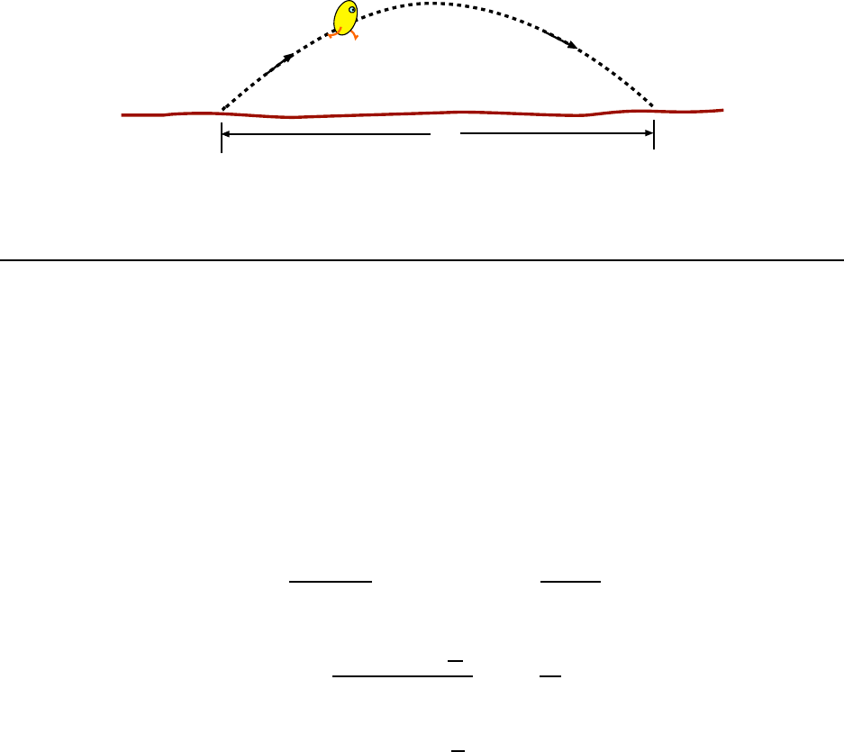
3.2. WORKED EXAMPLES 47
R
Figure 3.10: For the purpose of doing Example 9, treat the jumper as a small obj ect.
9. An Olympic long jumper leaves the ground at an angle of 23
◦
and travels
through the air for a horizontal distance of 8. 7 m be fore landing. What is the
takeoff speed of the jumper? [CJ6 3-33]
Even though a jumper is not a small object, for the purpose getting an answer we will
treat him/her as a “particle” which is launched from ground level (by its tiny legs!?!), moves
through the ai r and then lands at ground level. See Fig. 3.10.
So this is a problem where the projectile (the j umper) begins and ends at the same
height so we can use the results of the se ction where we got the results f or the range R. We
rearrange the result for R (Eq. 3.12) to solve for the initial speed v
0
:
R =
v
2
0
sin 2θ
0
g
⇒ v
2
0
=
Rg
sin 2θ
0
Plug in the numbers:
v
2
0
=
(8.7 m)(9.80
m
s
2
)
sin(46
◦
)
= 119
m
2
s
2
So then
v
0
= 11
m
s
48 CHAPTER 3. MOTION IN TWO DIMENSIONS
Chapter 4
Forces I
4.1 The Important Stuff
4.1 .1 Introduction
The preceding two chapters dealt with the mathematics of motion, kinematics. We now
begin the study of the physical reasons for the motion of objects, i.e. the study of dynamics.
Dynamics gives us the ability to predict the motion of an object in a particular physical
situation.
All motion around us can be found from an applicati on of three simple laws discovered by
Isaac Newton. These laws rel ate the influences which govern the motion of objects (forces)
to t he accelerations of the objects and to a prope r ty of these objects, their mass.
The three laws are simple to state but can take years to learn how to use, and that is
what makes physics a challenging (and interesting) subject. They were found to be adequate
for descr ibing all motion in the universe until early i n the 20th century, when they were
generalized by Albert Einstein to include motion at very large speeds and later by a bunch
of Germans to de al with moti on on the atomic scale.
Some word usage: Throughout the next few chapters we will b e talki ng about the motion
of objects whose sizes are “small” compared to the distance over which they are moving. In
that case, the fact that they may be rotating will not be important and we will just discuss
their overall motion. When we can treat motion in this way we will refer to the objec t as a
particle.
This chapter is a long one, because in it we encounter the basis of all (classical) physical
as well as examples of their usage. It is important to l ook at many examples of how we work
with forces; only then can you get the hang of doing physics.
49

50 CHAPTER 4. FORCES I
4.1 .2 Newton’s 1s t Law
Newton’s First Law (for our purposes) is based on earlier ideas by Galileo; it tells us what
happens if we don’t have any forces around, and states:
When there are no forces acting on an object its velocity remains the same.
This law contradicts “common sense” bec ause we are used to all motion coming to a halt
if we don’t do anything to maintain it. But common experience can be deceptive, and it
took the genius of Galileo and Newton to see that there are force s of friction which act on
everyday objects to slow them down. Take away such influences and the moti on (velocity)
continues forever, unchanged.
4.1 .3 Newton’s 2nd Law
When t here are influences (forces) acting on an object, then in general the velocity of the
object will change, that is, there will be an acceleration. Newton’s 2nd law tells us how to
find that acceleration. Knowing t he acceleration, we can predict the motion of the object,
as c overed in the preceding chapters.
When there is a stronger force acting on the objec t the acceleration is greater. So the
acceleration is proportional to the force: a ∝ F .
But it is also true that a given force doesn’t affect all objects in the same way. If an
object has more “bulk” to it, the accele r ation it unde rgoes will be smaller; in other words a
given force do esn’t do as well in changing the motion of a bulky object. The proper name
for property we are considering is mass; it is denoted by m and it is measured in kilograms.
Anyway, the acceleration is inversely proportional to the mass of the object: a ∝
1
m
Combining these two ideas, acceleration is proportional to force divided by mass: a ∝
F/m. Mul tiplying both sides by m gives the simple expression of Newton’s 2nd law:
F = ma
but we aren’t done yet.
First, force and acceleration are both vectors; they have direction and magnitude. Sec-
ondly, in general there may be several forces acting on a mass m. When there are, we take
the vector sum of these forces to get the total (net) force :
F
net
= F
1
+ F
3
+ F
3
+ . . .
and it is the net force that gives the acceleration of the object. Now we are prepared to state
Newton’s 2nd law:
4.1. THE IMPORTANT STUFF 51
When forces F
1
, F
2
, . . . act on a mass m, the acceleration of the mass can be
found from:
F
net
= ma . (4.1)
The equation in the 2nd law is a vector equation so it means the same thing as when we
write out the x and y components separately:
F
net, x
= ma
x
and F
net, y
= ma
y
(4.2)
4.1 .4 Units and Stuff
Mass is measured in kilograms. From the equation F = ma, we see that the units of force
F must be those of mass times those of acceleration,
Units of force = kg ·
m
s
2
=
kg · m
s
2
The combination of the basic SI units is known as the “newton”, in honor of you–know–who.
Thus:
1
kg·m
s
2
= 1 newton = 1 N
The SI unit of force is the newton; sometimes we see another units of force, the dyne:
1 dyne = 1
g·cm
s
2
= 10
−5
N
In the old “English” system of units (which we don’t use in this b ook) the units of force
is the pound, abbreviated as “lb” for reasons I’ll never understand. The relation with the
newton is:
1 lb = 4.448 N
4.1 .5 Newton’s 3rd Law
The third law of Newton is sometimes useful to us when we solve more complicated physics
problems. It says something profound about nature. And it is often mis-stated and misun-
derstood.
Newton’s Third Law says that when there is a f orce acting on a particle it must be due
to the presence of some other particle(s). Forces must co me from other objects. For there to
be a (real ) force acting on an object you have to be able to say what kind of object it might
come f r om.
Secondly, if there are two objects A and B exerting forces on one another then those forces
are equal in magnitude and opposite in direction. Some examples are shown in Fig. 4. 1.
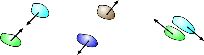
52 CHAPTER 4. FORCES I
A
B
F
B on A
F
A on B
A
B
F
B on A
F
A on B
A
B
F
B on A
F
A on B
(c)
(b)
(a)
Figure 4.1: Illustrations of Newton’s 3rd law. Force of A on B is “equal and opposite” to the force of B
on A.
So Newton’s 3rd Law is:
The force which object A exerts on object B is equal in magnitude and op-
posite in direction to the force which B exert s on A.
Note that this law has to do with forces; the objects may b e in motion or they may not
be, but the law only tells us about forces.
Unfortunately many people who think t hey understand physics expre ss the law something
like:
For every action there is an equal and opp osite reaction
This is a poor expression of the law because we never deal with anything prope rly called
“action” in this course, whi ch (to my m ind anyway) would seem to involve motion. It is
important to understand that the third law is about forces, and the se (“equal and opposite”)
forces are exerted on two different objects.
4.1 .6 The Force of Gravity
We discussed a very important example of acceleration in the last chapter – the acceleration
of a projectile – and we c an now relate that to a force.
The acceleration of a projec tile of mass m near the surface of the earth has magnitude
g and is directed downward. Then from F = ma, there is a force on the projectile with
magnitude mg and is dir ected downward. This is the force gravity; but where do es it come
from? (By Newton’s 3rd law, it must come from another object.)
That other object is the entire earth. The way this comes about was also disc overed
by Newton. He found that all masses in the universe attract one another with a force that

4.1. THE IMPORTANT STUFF 53
m
1
m
2
F
F
Figure 4.2: Ma sses m
1
and m
2
exert an attractive gravitational force on one another.
depends on the values of the masses and the distance between them; the mathematical
expression is his Law of Gravit ation.
The basic law of gravitation applies to two masses (m
1
and m
2
) whose si zes are small
compared to their separation (i.e. “point” masses). They are separated by a distance r. As
shown i n Fig. 4.2, each experiences an attractive force of magnitude F whose direction is
toward the position of the other mass and whose magnitude is
F = G
m
1
m
2
r
2
where G = 6.67 × 10
−11
N·m
2
kg
2
(4.3)
The number G is called the gravitational constant. Since the newton can be expressed
in te r ms of kg, m, and s, G can also be expressed as
G = 6.67 × 10
−11
m
3
kg·s
2
(4.4)
There is a gravitational force of attraction b etween any two objects but for everyday
objects this force is too small to be of any importance. However if one of the objects is
enormous —like a planet— then the force is not so small. The force of attraction between
a 1 kg mass and the entire earth is not small.
The problem is in how we calculate the attractive force between the earth and a small
object on its surface. It is reasonable that we should use m
1
= M
earth
and m
2
= m
object
in
Eq. 4.3, but what should we use for the di stance of separation r?
It turns out that it is exactly true that since the earth is a spherically symmetric sort of
thing, the proper distance to use in Eq. 4.3 is the distance between t he object and the center
of the earth, R
earth
; see Fig. 4.3.
Thus the magnitude of the force of gravity on an object of mass m is
F
grav
= G
M
earth
m
R
2
earth
=
GM
earth
R
2
earth
!
m
But wait! Earlier we said that the force of gravity on an object had to be mg, or gm:
F
grav
= (g)m
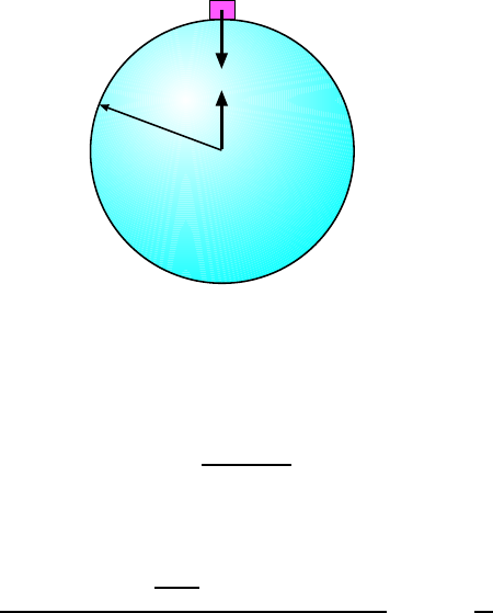
54 CHAPTER 4. FORCES I
F
F
R
earth
Figure 4.3: Earth exerts force F on object on its surface. For the r in Newton’s law, use R
earth
.
Since both are true, thi s can only mean that
g =
GM
earth
R
2
earth
(4.5)
Plugging in the numbers, we can see that we do get the value of g we’ve come to know and
love:
g =
(6.67 ×10
−11
N·m
2
kg
2
)(5.98 × 10
24
kg)
(6.38 × 10
6
m)
2
= 9.80
m
s
2
and we se e how the numerical value of g depends on the m ass and siz e of the earth. We
will get a different value for the accele ration of gravity on the surface of another planet, and
Eq. 4.5 shows us how to c alculate it.
Anway. . . when we consider the forces acting on any object on the surface of the earth,
we must include the force of gravity, which is called the weight of the obj ect, which, if the
object has mass m, has magnitude mg and is directed downward.
4.1 .7 Other Forces Which Appea r In Our Problems
In order to make use of knowledge of forces, we will be solving lots and lots of problems
involving simple things l ike blocks and strings and pulleys and inclined planes. We will
be calculating the forces exerted on the masses (when we know their acceleration) or the
acceleration of the masses (when we know the forces exerted on them.) Solving force problems
is the real guts of a physics course!
These objects will be idealized in the sense that we wil l approximate their behavior with
a simple rule . A real pi ece of stri ng or a real pulley won’t behave exactly in the way we’ll
use; the real behavior is more complicated and difficult.
The objects we’ll see are:
• String (c ord, rope) A string may be attached to a mass or a wall as in Fig. 4.4(a) or
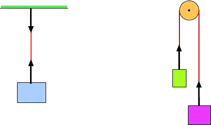
4.1. THE IMPORTANT STUFF 55
T
T
T
T
(a)
(b)
Figure 4.4: A string pulls inward along its length with a force of magnitude T .
it may be looped over a pulley, as in Fig. 4.4(b). The string will usually b e under tension.
When we are told this, it means that the string is pulling inward a t both ends on whatever is
attached with a force of magnitude T . Then T i s called the tension in the string. (Tensi on
is a scalar, and it has unit s of force, newtons.)
This is also true when the string is looped over an ideal, m assless pulley, i.e. the tension
is the same on both ends. Later though, we will deal with pulleys which have mass and this
won’t be true. For now, it is.
• Smooth Surface A mass may be in contact with a ”smooth surface”. We can approximate
such a surface by coating it with Teflon or spraying WD–40 all over it or possibly by putting
very small but i deal wheels on the block. A clever lad like you can think up something.
No real surface behaves this way because there will be a friction force between the
surface and the mass, but we’ll deal with that in t he next chapter.
The force from a smooth surface is perpendicular t o the surface. The magnitude of this
force wil l depend on whatever is going on in the problem. This f orce is called the normal
force of the surface just because in math, “normal” means “perpendicular”.
As mentioned, in the next chapter we will deal with surfaces which are m ore realisti c;
for these there is a frictional force which points along the surface. But not yet; for now, the
force is all normal (perpendicular).
When a mass slides on such a surface we note that its velocity and acceleration must
always point along the surface, that is, the r e will be no component of v or a perpendicular
to the surface. Since the acceleration has no component perpendicular to the surface, the
component of the net force perpendicular to the surface must also be zero. We will use this
fact in solving some problems involving hard surfaces.
• Spring scale Sometimes a problem will fe ature a scale. The innards of the device may
not be specified but we usually mean that there’s a spring of some sort inside. Two kinds of
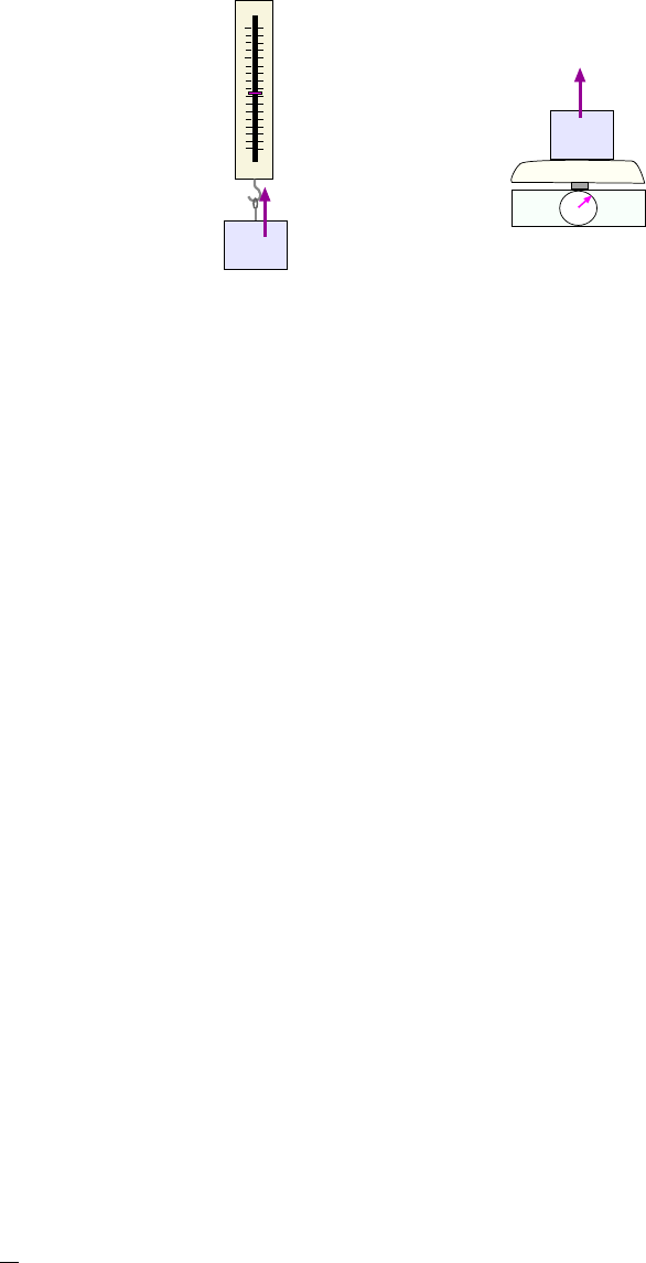
56 CHAPTER 4. FORCES I
(a)
(b)
F
scale
F
scale
Figure 4.5: Spring scales; the spring inside the device is under some tension and pull s or pushes on the
mass which is in contact with the scale. The magnitude of the force, F
scale
is in general not equal to the
weight of the mass!
spring scale are illustrated in Fig. 4.5. In each case the scale (or actually the spring inside of
it) exerts a force on the mass with which it is in contact, and the magnitude of this force is
what we read from the numerical scale on the device. In gener al, this value is not the same
as the weight mg of the mass! The scale reading will depend on the details of the problem
we are solving.
4.1 .8 The Free–Body Di agram: Draw the Damn Picture!
In general there will several kinds of forces acting on a mass in our problems. By Newton’s
Second law we have to find the (vector) sum of all these force in order to get the (vector)
acceleration. We will need a diagram of the directions of all the forces in order to add the
vectors correctly; i t’s also a good to organize our thinking by noting down al l the forces
explicitly, since that may help us see if we’ve omitted any forces (or included some that
shouldn’t be there).
So it is always a good idea to draw a sketch showing the mass and the force vectors which
act on it. Such a diagram goes by the fancy name of free–body diagram, but it amounts
to nothing more than drawing a damn diagram of the problem (with the forces specified)!
An example is given in Fig. 4.6. In (a) we have the physical situation of the mass; in (b)
we isolate the mass but show the directions of the forces acting on it.
4.1 .9 Simple Example: What Does the Scale Read?
To start with a simple example, we consider a 2.0 kg m ass hanging from a spring scale inside
an elevator, as shown in Fig. 4.7(a). Presently, the elevator is accel erating upward at a rate
of 1.80
m
s
2
. What is reading on the scale?
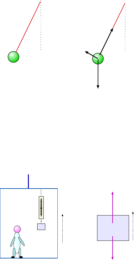
4.1. THE IMPORTANT STUFF 57
T
mg
F
air
(a) (b)
Figure 4.6: (a) A physics problem. (b) A free–body diagram for this problem.
a
m
m = 2.0 kg
a = 1.8 m/s
2
m
mg
F
scale
(a)
(b)
a
Figure 4.7: (a) Mass hangs from a scale inside an elevator which i s accelerating upward. (What does the
scale read?) (b) Forces acting on the mass.
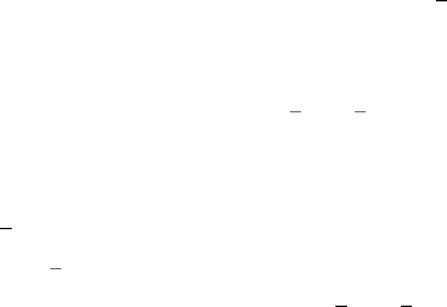
58 CHAPTER 4. FORCES I
It is true that if a mass m simply hangs from a scale and is not accelerating then the
upward force of the scale F
scale
will equal the downward force of gravity mg, and that is
because the force vectors must add up to give zer o for that case. But here the mass is
accelerating along with the el evator and all its contents so there is a net force and the force
vectors do not add up to zero.
In Fig. 4.7(b) we show the forces acting on the mass. Taking “up” as the +y direction,
the net force on the mass is
F
net, y
= F
scale
− mg
and from Newton’s 2nd law this is eq ual to ma
y
, wi th a
y
= +1.80
m
s
2
. Thus:
F
net, y
= F
scale
−mg = ma
y
=⇒ F
scale
= mg + ma
y
= m(g + a
y
)
Now plug in the numbers and get:
F
scale
= (2.0 kg)(9.80
m
s
2
+ 1.80
m
s
2
) = 23.2 N
So the force of the scale (the same as the t ension in its spring here) is greater than the value
of its weight, mg = 19.6 N. The scale will read 23.2 N. One way to express this result is to
say that the apparent wei ght of the mass is 23.2 N for the case we considered.
Now suppose t he elevator car is accelerating d ownward with an acceleration of magnitude
1.80
m
s
2
. What is the tension in the scale’s spring now?
The only thing that differs from the analysis we just did is the value of a
y
. Now we have
a
y
= −1.80
m
s
2
. This time we get
F
scale
= m(g + a
y
) = (2.0 kg)(9.80
m
s
2
−1.80
m
s
2
) = 16.0 N
so here the f orce from the spring is 16.0 N so that is what the scale will read. Here the
apparent weight of the mass is 16.0 N.
4.1 .10 An Important Example: Mass Sliding On a Smooth In-
clined Plane
An important example of the applying the principles for solving force proble ms is the case of
a mass (or rather, a block of mass m) sliding on a frictionless inclined plane which is sloped at
angle θ from the horizontal. The situation is shown in Fig.4.8. Note, we could be considering
a mass which is sliding down the plane and moving faster and faster, or where the veloc ity
of the mass is up the plane and its speed is decreasing. In either case the acceleration of t he
mass points down the slope and we would like to find i t s magnitude.
The first step is to identify the forces which act on the block. There are only two: One
is the force of gravity, which has a magnitude mg and points straight down. The other is
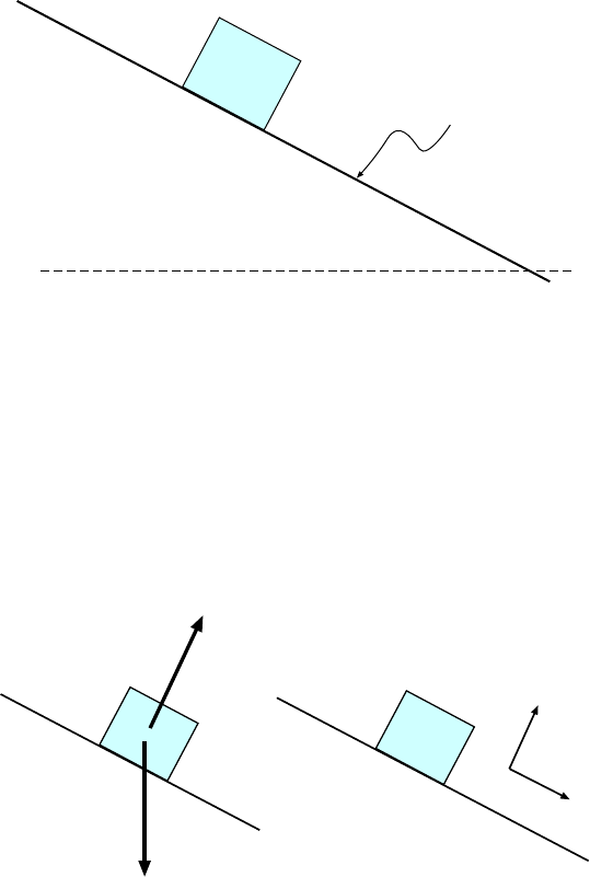
4.1. THE IMPORTANT STUFF 59
q
m
smooth!
Figure 4.8: Mass m on a frictionless inclined plane. Angle of incline is θ.
mg
F
N
y
x
(a)
(b)
Figure 4.9: (a) Forces which act on the mass on the inclined plane. (b) We use a coordinate system with
axes along the plane (x) and perpendicular to it (y).
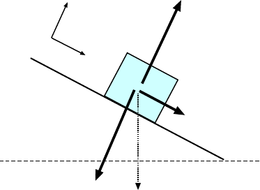
60 CHAPTER 4. FORCES I
mg
F
N
mg sin q
mg cos q
q
y
x
Figure 4.10: The force of gravity (downward, mg) has the indicated components in our new coordinate
system.
the normal force of the surface which points perpendicular to the surface, with a magnitude
we’ll call F
N
. These are shown in Fig. 4.9(a).
The next steps involve some reasoning and math that are a little tricky, but it important
to understand them. The one thing we know about the mass is that its motion must take
place along the slope of the plane. The component of its acceleration perpendicular to the
plane is zero. Therefore it will be to our advantage to use a coordinate system which has axes
along the plane (x, dire cted down the plane) and perpendicul ar to it (y). These are shown
in Fig. 4.9(b). So now the normal force F
N
points along +y but the force of grav ity points
along neither x nor y. That’s okay— we can get its x and y components in the new system
and work with those instead of the original vector. One can show with some geometry that
the component along the slope has magnitude mg sin θ and the one along y (going i nto the
plane) has magnitude mg cos θ. These components are illustrated in Fig. 4.10.
As we said, the y component of the total force must be zero. This gives us:
F
N
−mg cos θ = 0 so F
N
= mg cos θ
so (for what it’s worth) we know the magnitude of the normal force from the surface. Later
on, we will need this result.
The total force in the x direct ion is not zero, and Newton’s 2nd Law gives us:
mg sin θ = ma
x
but the mass m cancels on both sides, giving us
a
x
= g sin θ
The acceleration of the mass is dir ected down the slope (as we would expect ) and it has
magnitude mg sin θ. (It is a positive number because we had our x axis point do wn the
slope .
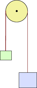
4.1. THE IMPORTANT STUFF 61
m
1
m
2
Figure 4.11: Attwood machine; if released from rest, bigger mass goes down and the smaller mass goes
up!
Note that it gives the right values at θ = 0
◦
(namely, a
x
= 0) and at θ = 90
◦
(namely
a
x
= g).
4.1 .11 Another Impo rtant Example: The Attwood Machine
The so–called Attwood Machine consists of two masses m
1
and m
2
joined by a string which
passes over a pulley. As we will treat it in this example the pull ey and string are massless
and ideal. Such a device is shown in Fig.4.11. If we suppose that m
2
is greater than m
1
(we
don’t lose any “generality” if we do that; we’re always free to call the larger mass “m
2
”) then
if the masses are released, m
2
will accelerate downward while m
1
will accelerate upward. We
should be very surprised if m
1
went downward!
We would like to find the value of the accelerations of the masses and also the tension in
the string.
In this problem there are two masses so we must analyze the forces (with diagrams)
on both of them individually. We begin with m
1
. The forces acti ng on m
1
are shown in
Fig.4.12(a). The string tension T goes upward; the force of gravity m
1
goes downward. Now
here we expect m
1
to move upward so we’ll let the coordinate axis y go upward as usual and
let a be the component of its upward acceleration. Then applying Newton’s 2nd law i n the
y direction gives
T − m
1
g = m
1
a (4.6)
Now we move on to m
2
. But b efore thinking about the forces on m
2
we can think about
its motion. We expect the acceleration to be downward but we note that since m
1
and m
2
are connected by a taut string their motions are related. In particular at any given time
their speeds are equal and the rates of changes of the se speeds are the same. That implies
that the magnitudes of their accelerations are equal. If m
1
has an acceleration a upward , m
2
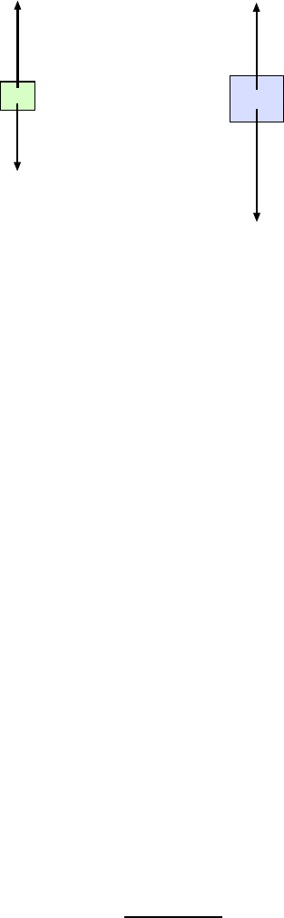
62 CHAPTER 4. FORCES I
m
1
m
2
T
m
1
g
T
m
2
g
(a)
(b)
Figure 4.12: (a) Forces o n m
1
in the Attwood machine. (b) Forces on m
2
in the Attwood machine.
will have an acceleration a downward. It wi ll be easier for us (I think) to use a downward
coordinate for m
2
; then the sum of the downward forces will give m
2
a, by N ewton’s 2nd law.
So now we look at the forces on m
2
, shown in F ig. 4.12(b). Gravity m
2
goes downward
and the string tension T (same tension on both ends) goes upward. Newton’s 2nd law gives:
m
2
g − T = m
2
a (4.7)
Now, taking m
1
and m
2
as “known” values, the two things we don’t know are a and T ,
and we want to find these. Eqs. 4.6 and 4.7 are two e quations for these two unknowns so we
can use algebra to solve for them. If write them together:
T − m
1
g = m
1
a
m
2
g − T = m
2
a
then add the corresponding left and right sides we cancel the te nsion T to get:
m
2
g − m
1
g = m
1
a + m
2
a
factoring both sides gives
(m
2
− m
1
)g = (m
1
+ m
2
)a
and finally, dividing both sides by (m
1
+ m
2
to isolate a gives
a =
(m
2
−m
1
)
(m
1
+ m
2
)
g (4.8)
We can check this result by consideri ng two simple cases:
• If the masses are equal, m
1
= m
2
, then Eq 4.8 gives a = 0, as we expect; with equal masses
there is no acceleration. However in that case the masses may still have a velocity.
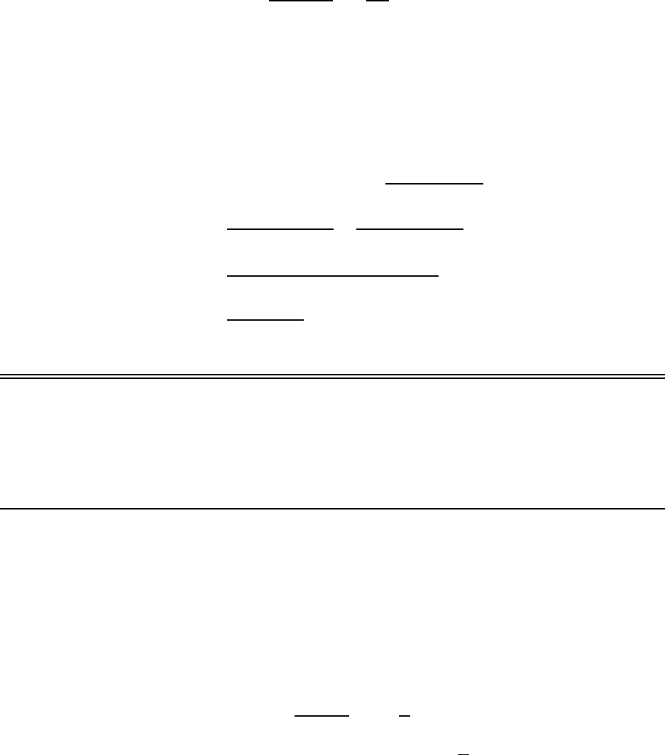
4.2. WORKED EXAMPLES 63
• If m
1
(the smaller mass) is z ero, then 4. 8 gi ves
a =
(m
2
− 0)
(0 + m
2
)
g =
m
2
m
2
g = g
so m
2
falls down with the same acceleration it would have if we just dropped it. But is
essentially what i s happening here since we are taking m
1
and the string as having no mass.
So this case gives the c orrect answer as well.
Now we find the te nsion in the string. We can use Eq. 4.6, substitute the expression for
a and do some algebra:
T = m
1
g + m
1
a = m
1
g +
m
1
(m
2
− m
1
)
(m
1
+ m
2
)
g
=
m
1
(m
1
+ m
2
)g
(m
1
+ m
2
)
+
m
1
(m
2
− m
1
)g
(m
1
+ m
2
)
=
(m
2
1
+ m
1
m
2
+ m
1
m
2
− m
2
1
)g
(m
1
+ m
1
)
=
2m
1
m
2
g
(m
1
+ m
2
)
4.2 Worked Examples
4.2 .1 Newton’s Second Law
1. Forces act on a 4.0 kg mass, as shown in Fig. 4.13. Find the magnitude and
direction of the acceleration of the mass when forces are as shown in (a) and (b).
(a) Here there is a single force acting in the +x direction, so the net force is given by
F
net, x
= +5.0 N. Put this into Newton’s 2nd law:
F
net, x
= ma
x
=⇒ 5.0 N = (4.0 kg)a
x
Solve for a
x
:
a
x
=
(5.0 N)
(4.0 kg)
= 1.2
m
s
2
The acceleration is in the +x dir ection and has magnitude 1.2
m
s
2
.
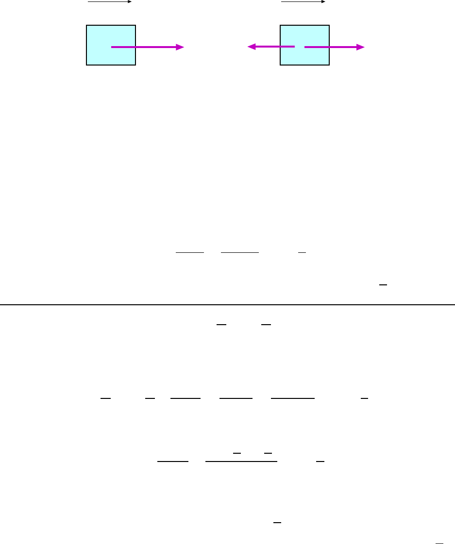
64 CHAPTER 4. FORCES I
4.0 kg
5.0 N
x
(a)
4.0 kg
3.0 N
x
(b)
2.0 N
Figure 4.13: Forces a ct on a 4.0 kg mass in Example 1.
(b) Here we have to add two force vectors together; the forces are both directed along the
x axis (one of them points in the −x direction) so the total x−force is
F
net, x
= +3.0 N − 2.0 N = +1.0 N
And this time Ne wton’s 2nd law gives us:
a
x
=
F
net, x
m
=
(1.0 N)
(4.0 kg)
= 0.25
m
s
2
The acceleration of the mass is in the +x direction and has m agnitude 0.25
m
s
2
.
2. A car accelerates uniformly from 0
mi
hr
to 70
mi
hr
in 9.50 s. During this time what
is the force on the 80 kg driver?
First, find the final speed of the car in sensible units! We have:
70
mi
hr
= (70
mi
hr
)
1 hr
3600 s
!
5280 ft
1 mi
!
0.3048 m
1 ft
= 31.3
m
s
So the acceleration of the car is
a
x
=
v − v
0
t
=
(31.3
m
s
− 0
m
s
)
(9.5 s)
= 3.29
m
s
2
The acceleration of the driver is the same as that of the car! Newton’s 2nd law applied to
the driver gives
F
net x
= ma
x
= (80.0 kg) ( 3.29
m
s
2
) = 264 N
The force on the driver (horizont al ; he has no vertical acc eleration) has magnitude 264
m
s
2
.
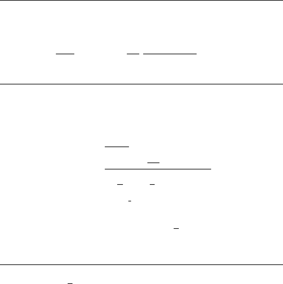
4.2. WORKED EXAMPLES 65
4.2 .2 The Force of Gravity
3. What is the magnitude of t he force of gravitational attraction between two
2.00 kg masses separated by 50.0 cm?
Use Eq. 4.3 with m
1
= m
2
= 2.0 kg and r = 0.500 m:
F = G
m
1
m
2
r
2
= (6.67 × 10
−11 N·m
2
kg
2
)
(2.00 kg)(2.00 kg )
(0.500 m)
2
= 1.07 ×10
−9
N
The force of gravity is 1.07 × 10
−9
N.
4. Mars has a mass of 6.46 × 10
23
kg and a radius of 3.39 × 10
6
m. (a) What is the
acceleration due to gravity on Mars? (b) How much would a 65 kg person weigh
on this planet? [CJ6 4-27]
(a) Use Eq. 4.5 using the mass and radius of Mars to get g
Mars
:
g
Mars
=
GM
Mars
R
2
Mars
=
(6.67 × 10
−11
N·m
2
kg
2
)(6.46 ×10
23
kg)
(3.39 × 10
6
m)
2
= 3.75
N
kg
= 3.75
m
s
2
So we get a value which a bi t more than
1
3
of the value of g on the Earth.
(b) The weight of an object of mass m on Mars is W
Mars
= mg
Mars
, so
W
Mars
= mg
Mars
= (65 kg)(3.75
m
s
2
) = 244 N
4.2 .3 Applying Ne wton’s Laws of Motion
5. A 3.00 kg mass is pulled upward by means of an attached rope such t hat its
acceleration is 2.20
m
s
2
upward. What is the tension in the rope?
The basic problem is illustrated in Fig. 4.14(a). The first thing to do is to note down
all the forces acting on the mass, and this done in the “free–body–diagram” in Fig. 4.14(b):
The rope tension T pulls upward and the force of gravity mg is directed downward (with
m = 3.00 kg).
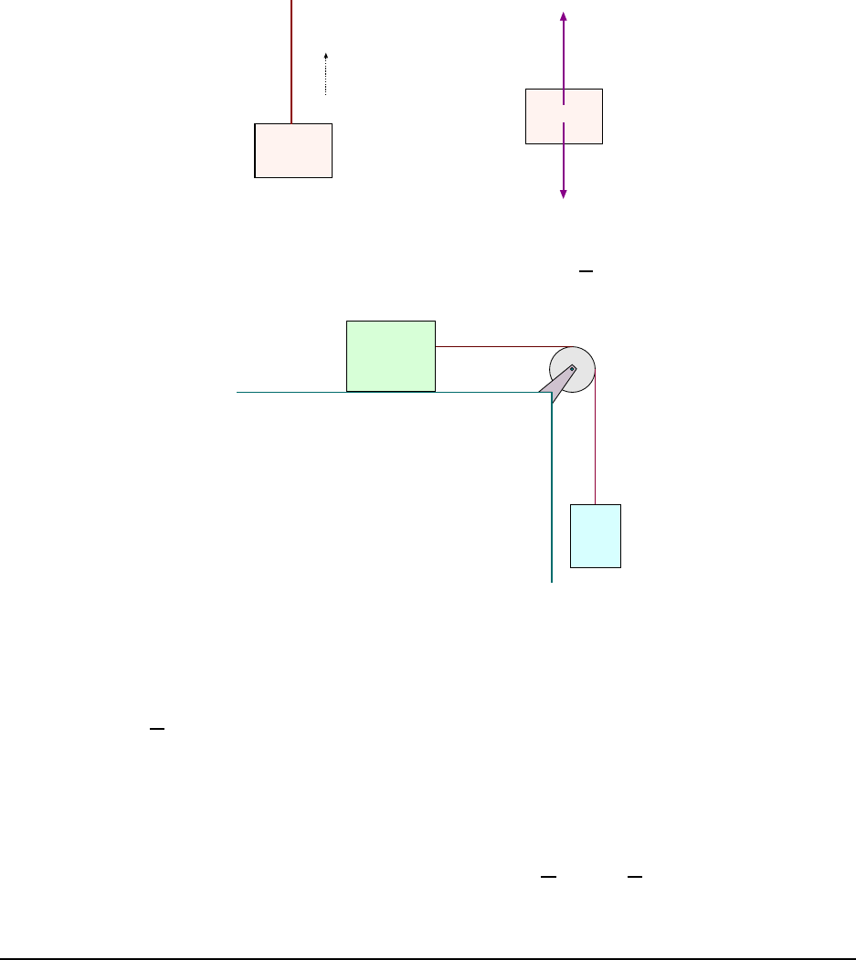
66 CHAPTER 4. FORCES I
3.0 kg
a = +2.2 m/s
2
mg
T
(a)
(b)
Figure 4.14: (a) Mass is pulled upward by a rope so that a
y
= +2.20
m
s
2
. (b) Free–body–diagram for the
mass.
m
1
m
2
m
1
= 3.0 kg
m
2
= 2.0 kg
Figure 4.15: Masses joined by a string, in Example 6. m
1
(3.00 kg) slides on a smooth surface. m
2
hangs
from the string and falls downward.
By Newton’ 2nd law, the sum of the forces must equal ma and here the acceler ation has
magnitude 2.20
m
s
2
and goes upward. So Newton’s 2nd law gives:
T − mg = ma
y
Solve for T :
T = mg + ma
y
= m(g + a
y
) = (3.00 kg)(9.80
m
s
2
+ 2.20
m
s
2
) = 36.0 T
The tension in the rope is 36.0 N.
6. A 3.00 kg mass slides on a smooth horizontal surface; it is joined by a string to
a hanging 2.00 kg mass. The string passes over a massless ideal pulley, as shown
in Fig. 4.15. When the 2.00 kg mass is released, (a) what is the acceleration of
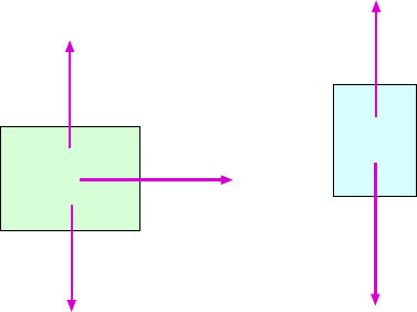
4.2. WORKED EXAMPLES 67
m
1
m
2
m
1
= 3.0 kg
m
2
= 2.0 kg
T
m
2
g
T
(a)
(b)
m
1
g
F
N
Figure 4.16: (a) The force(s) a cting on m
1
in Example 6. (b) the forces acting on m
2
.
the two masses? (b) What is the tension in the string?
(a) Before getting to the forces on the masses and the free–body–diagram, we ponder some
features of thi s problem. The 3.00 kg mass (to be called m
1
) will accelerate to the right
and the 2.00 kg mass (m
2
) will accel erate downward. These accelerations are in different
direct ions, but since the masses are joined by a string the distances they travel in any
amount of time are the same. So the magnitudes of their accel erations will be the same.
Now consider the forces acting on the masses. These are shown in Fig. 4.16. Mass m
1
experiences a f orce m
1
g downward from gravity, a force from the table F
N
(the “mormal
force”) upward and a force T from the string tension to the right. Now, this mass isn’t
moving up or down so the vertical forces have to sum to zero. This gives us
F
N
− m
1
g = 0 or F
N
= m
1
g
which is correct, but doesn’t help to solve the proble m.
The horizontal force on m
1
gives its accel eration (to the right) and by Newton’s second
law we have
T = m
1
a (4.9)
It is true that here m
1
= 3.00 kg, but it will be more useful to do some algebra first and
then plug in the numbers at the end.
Now we look at the forces on m
2
, as shown in Fig. 4.16(b). There is the string tension T
pulling upward and the f orce of gravity m
2
g pulling downward. Since we m ade the positive
direciton of m
1
’s motion to the r ight, it is consistent to make the direction of positive motion
for m
2
downward, so that is what we will do. In that case, the downward acceleration of m
2
is a, so adding up the downward forces on m
2
, Newton’s second law gives
m
2
g − T = m
2
a (4.10)
68 CHAPTER 4. FORCES I
Now we know the values of m
1
and m
2
and also the alue of g; the things we don’ t know
in Eqs. 4.9 and 4.10 are T and a and of these it’s really a that we want. Since we have two
equations for two unknown quantities, we can do some algebra and find both of them.
If we add the resp ective left and right sides of the two equations we will get another
(valid) equation. The reason for doing this is that the tension T wi ll cancel on the left side.
This gives:
T + m
2
g −T = m
1
a + m
2
a
A little algebra gives us
m
2
g = (m
1
+ m
2
)a
and the n we can isolate a:
a =
m
2
g
(m
1
+ m
2
)
. (4.11)
Plugging in the numbers for the particular masses, the common acceleration is
a =
(2.00 kg)(9.80
m
s
2
)
(3.00 kg + 2.00 kg)
= 3.92
m
s
2
(b) We now have a so we can use Eq. 4.9 to get T :
T = m
1
a = (3.00 kg)(3.92
m
s
2
) = 11.8 N
Chapter 5
Forces II
5.1 The Important Stuff
5.1 .1 Introduction
In this chapter we cover two more topics having to do with the basic applic ation of Newton’s
laws.
First we discuss the force of friction, specifically as it occurs when two soli d objects slide
against one another. This will allow us to solve more realistic problems and give us more
practice in making our force diagrams and applying Newton’s 2nd law.
Then we wil l discuss the special (but i mportant) case when a mass moves in a circle at
constant speed. As we will see, this calls for a careful understanding of the directions of the
forces and acceleration.
5.1 .2 Friction Forces
Now we need to go back to the examples of the last chapter and add a little realism.
We had some examples where a mass (i.e. a block) slides along a flat surface. Here we
want to take account of the f act that real surfaces are not smooth; in additi on to the force
perpendicular to the surface (the “normal force”) there is also a f orce parallel to the surface
which comes from friction forces.
How do we get the magnitude and direction of this friction force ? Alas, it is a bit tricky
but to have even the simplest discussion of friction we need to go into some details.
Sliding friction forces come in two kinds. In one kind, the bl ock is not moving over the
surface; a frict ional force is opposing some other app lied forces so that there is no net force
and the block does not move. This is a force of st atic friction from the surface.
Now if we apply larger and larger forces to the block eventually it will move. So the static
friction force can take on values up to some maximum value, which, in a given situation we’ll
69
70 CHAPTER 5. FORCES II
call f
Max
s
.
How can we find this maximal value? Empirically one finds that it depends on two things:
(!) The kinds of surfaces (materials) that are rubbing together. (2) The normal f orce between
the two surfaces. The maximal value is proportional to the normal force between the surfaces
(as we might expect; push them together harder and they stick together more) so the formula
for f
Max
s
turns out to be
f
Max
s
= µ
s
F
N
(5.1)
where F
N
is the normal force between the surfaces and µ
s
is a number which depends on the
types of surfaces which are in contact. µ
s
is called the coefficient of static friction and
since f
Max
s
and F
N
are both forces it doe sn’t have any units (i.e. it is pure number). I t is
very small when the surfaces are smooth and non–sticky.
The next kind of sliding friction happens when a block is moving over a rough surface.
Now there is a force of kinetic friction whose direction is opposite the direction of motion
and which has a magnitude f
k
. The magnitude of this friction force is given by a rule similar
to the one which gave the maximum value of the static friction force. f
k
depends on the types
of materials in contact as well as the normal force between the two surfaces. Empirically,
one finds:
f
k
= µ
k
F
N
(5.2)
where the number µ
k
is a unitless constant called the coefficient of kinetic fricti on.
Note how Eq. 5.2 is different from Eq. 5.1. Eq. 5.2 gives the actual value of the force of
kinetic friction whereas Eq. 5.1 just tells us how large the static friction force can possibly
be; its specific value will depend on the details of the other forces acting on t he mass.
5.1 .3 An Important Example: Block Sliding Down Rough Inclined
Plane
We go back to an “Important Example” considered in the last chapter, that of a block sliding
down an inclined plane. In that chapter we assumed the plane was perfectly smooth; what
happens if the plane is rough, with a coefficient of kinetic friction µ
k
?
The first thing to do is to make a diagram of the forces acting on the block. In Fig. 5. 1(a)
we show the forces which act on the block. Gravity with magnitude mg points downward.
The normal f orce of the surface points outward from the surface with magnitude F
N
. And
now there is a force of kinetic friction which is directed opposite to the motion with magnitude
f
k
. We’ve said that the bl ock will be sliding down the slope so the friction force points up
the slope.
Once again, t here is only motion along x so there can be no net force in the y direction.
This gives us
X
F
y
= F
N
− mg cos θ = 0 =⇒ F
N
= mg cos θ (5.3)
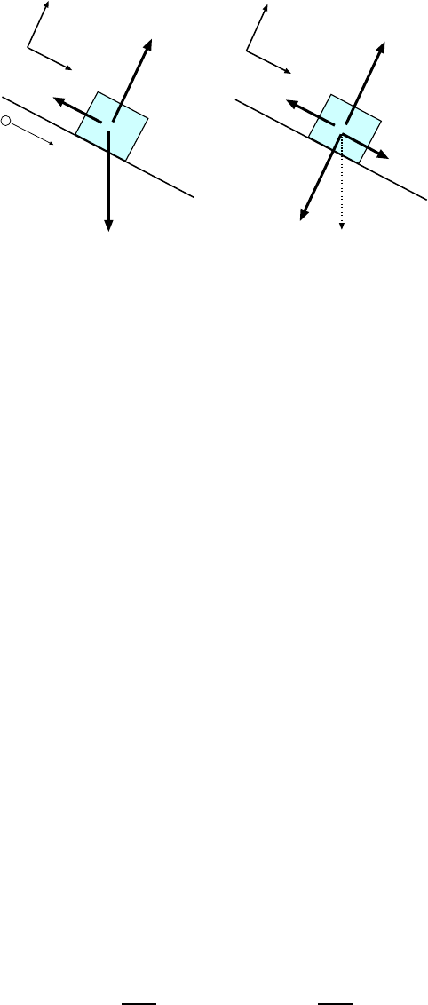
5.1. THE IMPORTANT STUFF 71
mg
F
N
y
x
(a)
(b)
mg sin q
F
N
fk
mg cos q
mg
y
x
+
Dir. of motion
fk
Figure 5.1: Block sliding down a rough inclined plane. (a) Basic forces acting on the block . (b) Again, it
is useful to get the components of the gravity force a long x and y.
and by Newton’s 2nd law the sum of the x forces gives
X
F
x
= mg sin θ −f
k
= ma
x
. (5.4)
From the last chapter we know that f
k
= µ
k
F
N
and using Eq. 5.3 we get
f
k
= µ
k
= µkmg cos θ (5.5)
Now using this in Eq. 5.4 we get
mg sin θ − µ
k
mg cos θ = ma
x
.
We can cancel the mass m from both sides to get
a
x
= g sin θ − µ
k
g cos θ (5.6)
It is interesting that once again the acceleration down the slope does not depend on the
mass, but it does depend on the types of surfaces involved, through the coefficient of friction
µ
k
.
5.1 .4 Uniform Circular Motion
We consider an important kind of motion not covered in Chapter 3. This is where a particle
moves in a circular path (with radius r) with constant speed, v, as shown in Fig. 5.2.
Suppose it takes a time T for the particle to go around the c ircle . Since it then moves a
distance C = 2πr in a time T , the speed of the particle must be
v =
2πr
T
⇒ T =
2πr
v
(5.7)
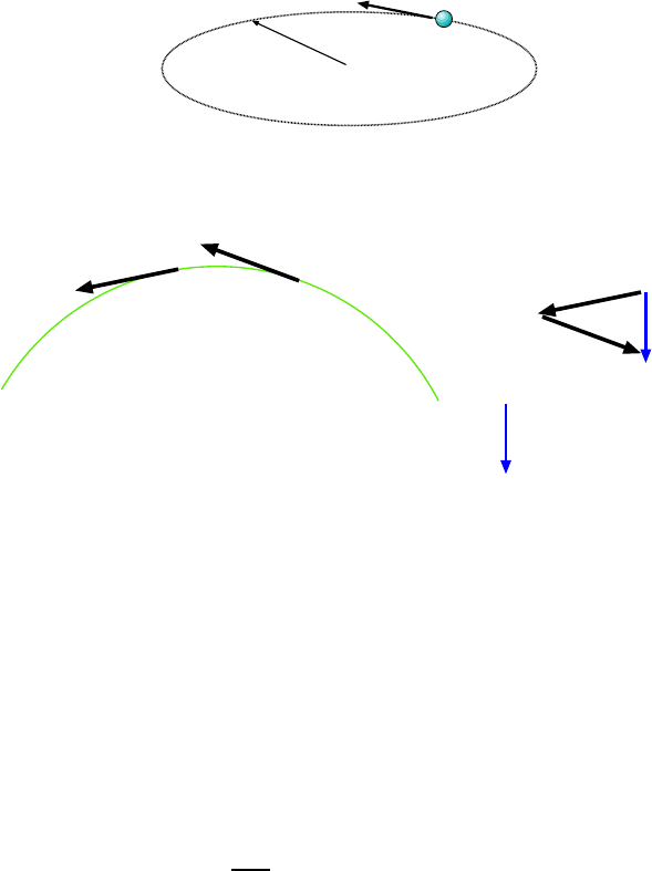
72 CHAPTER 5. FORCES II
v
r
Figure 5.2: Uniform circular motion.
v
1
v
2
-v
1
v
2
Dv
Dv = v
2
- v1
(a)
(b)
Figure 5.3: (a) Velocity vectors at two different times. (b) ∆v gives the direction of the acceleration vector.
Next , some questions to te st our understanding of velocity and acceleration: Is this a
case of constant velocity? It is not. Even though the velocity of the particle al ways has the
same magnitude, the direction of the vel ocity is changing, and that is important. So the
particle has an acceleration and a net force which gives that acceleration.
What is the direc t ion of this acceleration? To find the answer we have to go back to the
basic definition of the acce leration vector; it is the rate of change in the veloc ity vector, i.e.
a =
∆v
∆t
for very small ∆t
We consider the difference in velocity vectors for two points on the particle ’s path which are
close together in time. This is shown in Fig. 5.3(a). Ve locity vectors at times t
1
and t
2
, v
1
and v
2
point very nearly in the same direction, but not quite! If we take the difference of
these two vectors, as shown in Fig. 5. 3(b), we find that ∆v = v
2
− v
1
points toward the
center of the ci rcle. Since to get the acceleration we just divide ∆v by the interval ∆t, the
acceleration must also point toward the center of the circle. Thus:
For uniform circular motion, the acceleration vector always points toward the center.
Because of this we say that the acceleration i s centripetal. We note that sinc e the
acceleration does not have the same direction all the time (though it does have the same

5.1. THE IMPORTANT STUFF 73
magnitude), the acceleration is not c onstant either!
What is the magnitude of the acceleration? One can show that the magnitude of the
acceleration is given by:
a
c
=
v
2
r
(5.8)
where r is the radius of the circle and v is the (constant) sp eed of the partic le. The subscript
“c” just indicates that this is the m agnitude of the centripetal acceleration.
5.1 .5 Circular Motion and Force
Newton’s 2nd law, F
net
= ma tells us something about the forces acting on a particle which
undergoes uniform circular motion. It says that the total force must also be pointing toward
the center of the circle and it must have a magnitude given by
F
c
=
mv
2
r
(5.9)
where again the subscript c indicates that the direction of the force is toward the center.
5.1 .6 Orbital Motion
Using the equations for uniform circular motion and Ne wton’s law of gravity we can under-
stand some features of the orbits of planets around the sun or of moons of the planets.
Consider a small mass m
2
in m otion around a much larger m ass m
1
; m
1
is l arge enough
that we will assume it is stationary. Mass m
2
experiences an attractive force toward m
1
and
we will consider the case where this force provides the centripetal force for motion of m
2
around m
1
in a circular orbit of radius r. m
2
is moving with constant speed v. See Fig. 5.4.
To repe at, m
2
moves around m
1
because at all times it is being pulled toward m
1
.
Since the distance between the two masses (their centers, actually) is r, the gravitational
force on m
2
is given by
F
grav
= G
m
1
m
2
r
2
and from the facts about its orbit, the t otal force on m
2
must be pointing toward the center
with magnitude
F
c
=
m
2
v
2
r
But the gravity force on m
2
is the total force on m
2
, so
F
grav
= F
c
=⇒ G
m
1
m
2
r
2
=
m
2
v
2
r
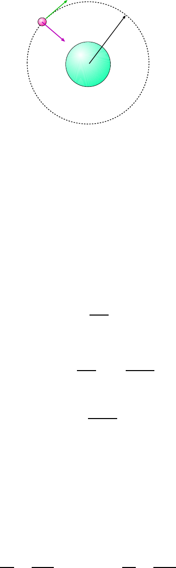
74 CHAPTER 5. FORCES II
r
m
2
m
1
v
F
grav
Figure 5.4: Small mass m
2
is in orbit around the much larger mass m
1
; we assume that m
1
doesn’t move
and that the orbit is a circle centered on the center of m
1
. The centri petal force on m
2
is the gravitational
force F
grav
.
We see that m
2
cancels in the last equation as does one power of r. We can write the result
as
Gm
1
= rv
2
(5.10)
There is a clearer way to express Eq. 5.10 because the things we usually know about a
planet or moon are the radius of the orbit r and the period of its motion, that is, the time
it takes to make one revolution, T . Since one re volution has a path length of 2πr, the speed
v and T are related by
v =
2πr
T
Put this into Eq. 5.10 and with a little algebra get:
Gm
1
= r
2πr
T
2
=
4π
2
r
3
T
2
which we can write as
T
2
=
4π
2
r
3
Gm
1
(5.11)
We note that that the mass of the small orbiting object m
2
does not appear in this equation;
so i t says that for any mass orbiting m
1
in a circular orbit, the period and orbital radius
are related as given in Eq. 5.11. It says that as r gets larger so does T , but the two are not
proportional; rather, the square of T is proportional to the cube of r.
Relation 5.11 is the modern version of a rule for planetary motion discovered by Kepl er.
Keple r considered the planets of the solar syste m which all orbit the same object, namely
the sun. If we consider two pl anets with individual radii and periods r
1
, T
1
and r
2
, T
2
, the n
Eq. 5.11 gives
T
2
1
r
3
1
=
4π
2
GM
and
T
2
2
r
3
2
=
4π
2
GM
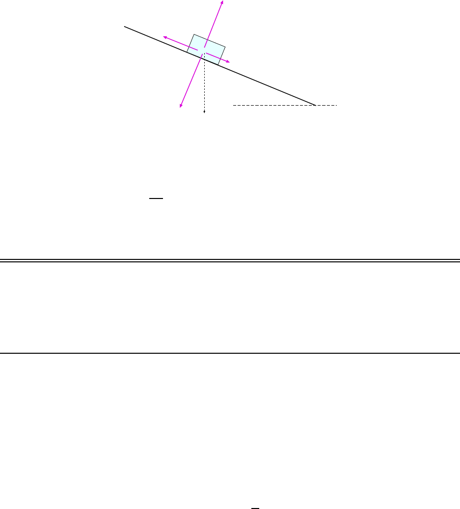
5.2. WORKED EXAMPLES 75
mg
mg sinq
mg cosq
q
q
q = 15
o
F
stat
N
m = 4000 kg
Figure 5.5: Forces acting on a 4000 kg truck is parked o n a slope.
where M is the mass of the sun. This tells us:
T
2
r
3
= the same for all pl anets (5.12)
We can use 5.12 to get the period or distance of a planet if we know both the period and
distance of another planet orbiting the same central object.
5.2 Worked Examples
5.2 .1 Friction Forces
1. A 4000 kg tr uck is parked on a 15
◦
slope. How big is the fri ction force on t he
truck? [KJF 5-26]
The forces which act on the truck are shown in Fig. 5.5. With m = 4000 kg and θ =
15
◦
, the downward force of gravity mg has been decomposed into components along and
perpendicular to the slope as we’ve done before. There is a normal force from the road with
magnitude N. The truck has no acceleration so there is no net force and so there must be
a f orce going up the slope, which of course is from static friction, denoted by F
stat
.
For the force s along the slope to cancel we must have
F
stat
= mg sin θ = (4000 kg)(9.80
m
s
2
) sin 15
◦
= 1.01 × 10
4
N
so that is the magnitude of the friction force.
What about Eq. 5.1? That equation only gives the maximum value t hat the force of
static friction can take on. No one said that this was the case in this problem . (The problem
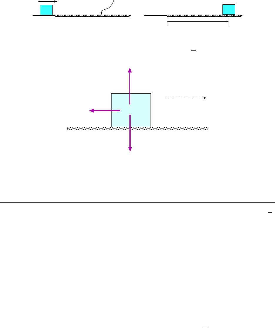
76 CHAPTER 5. FORCES II
2.80 m/s
m
m = 0.300
m
x
(a)
(b)
Figure 5.6: (a) Block is slidi ng on a smooth surface with a speed of 2.80
m
s
. It encounters a surface which
is rough, with µ
k
= 0.300. (b) Blo ck has come to a halt a fter moving a distance x on the rough surface.
m
mg
F
N
f
k
Dir. of motion
m= 0.500 kg
Figure 5.7: Forces acting on the mass in Example 2 while it is sliding on the rough surface.
did not say the truck is on the verge of slipping.) So while that equation is true, it’ s not
relevant to the problem .
2. A block of mass 0.500 kg slides on a flat smooth surface with a speed of 2.80
m
s
.
It then slides over a rough surface with µ
k
and slows to a halt. While the block is
slowing, (a) what is the frictional forc e on the block? (b) What is the magnitude
of the block’s acce leration? (c) How far does t he block slide on the rough part
before it comes to a halt?
The problem is illustrated in Fig. 5.6. As indicated in Fig. 5.6 the bl ock slides a distance
x in coming to a halt on the rough surface.
First, find the forces which act on the block... draw the damn picture, as we do in Fi g. 5.7.
The forces are gravity (mg, downward) the normal force from the surface (F
N
, upward) and
the force of kine tic fricti on (f
k
, backward i.e. opposite the direction of motion).
Now, the motion only takes place along a horizontal line, so the vertical acceleration is
zero. So the ne t vertical force on the mass is zero, givi ng:
F
N
− mg = 0 =⇒ F
N
= mg = (0.500 kg)(9.80
m
s
2
) = 4.90 N
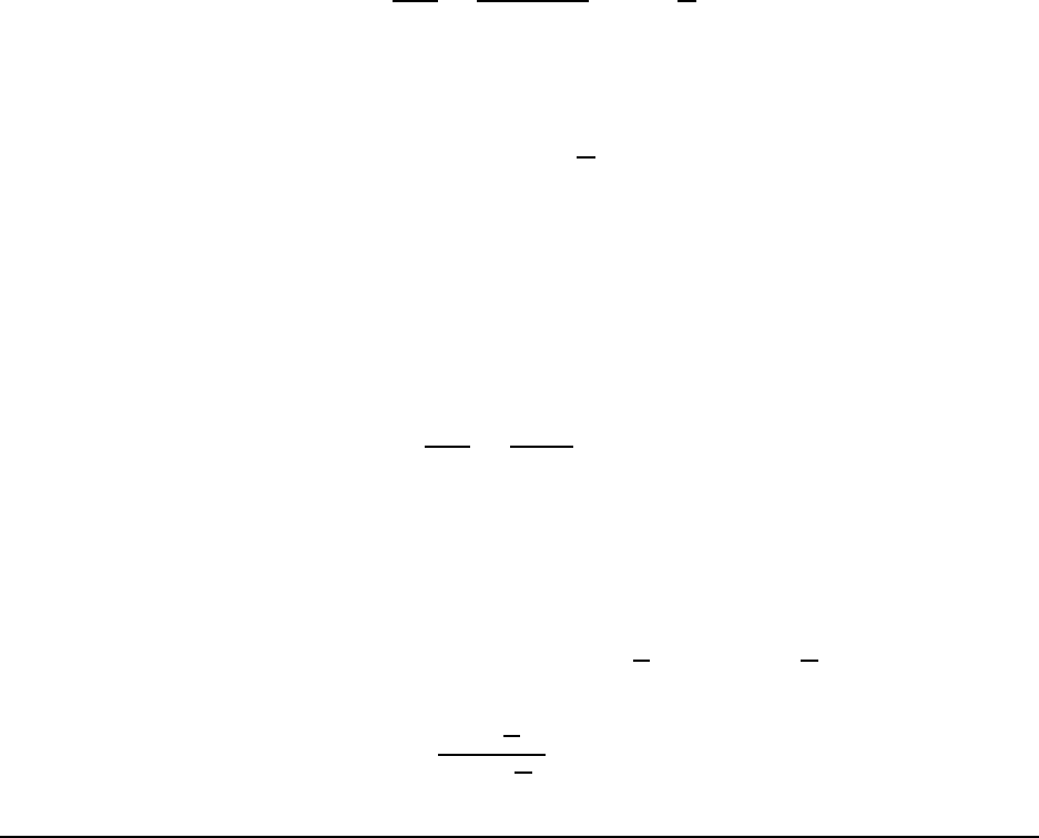
5.2. WORKED EXAMPLES 77
Now that we have the normal f orce of the surface, Eq. 5.2 gives us the m agnitude of the
(kinetic) friction force:
f
k
= µ
k
F
N
= (0.300)(4.90 N) = 1.47 N
(b) The net force on the block is the friction force so that the magnitude of the block’s
acceleration is
a =
F
net
m
=
(1.47 N )
(0.500 kg)
= 2.94
m
s
2
We should note that the direction of the acceleration opposes t he diretion of moti on, so if
the velocity is along the +x direction, the acceleration of the block is
a
x
= −2.94
m
s
2
Actually, by plugging the numbers i nto the formulae we’ve missed an important point.
Going back to part (a), we had F
N
= mg, so that
f
k
= µ
k
F
N
= µ
k
mg
and the magnitude of the acceleration is
a =
F
net
m
=
µ
k
mg
m
= µ
k
g ,
that is, the acceleration of the m ass does not depend on the value of m, just on µ
k
and g.
(c) The distance travelled by the mass bef ore it comes to a halt: We have the initial velocity
v
0
of the mass, the final vel ocity (v = 0) and the acceleration. We can use Eq. 2.8 to solve
for x:
v
2
= v
2
0
+ 2ax =⇒ 0
2
= (2.80
m
s
)
2
+ 2(−2.94
m
s
2
)x
Solve for x:
x =
(2.80
m
s
)
2
2(2.94
m
s
2
)
= 1.33 m
3. A block slides down a rough incline sloped at an angle of 40.0
◦
from the
horizontal. St arting from rest, it slides a distance of 0.800 m down the slope in
0.600 s. What is the coeffi cient of kine tic friction for the block and surface?
The problem is illustrated in Fig. 5.8. From the information gi ven about the motion of
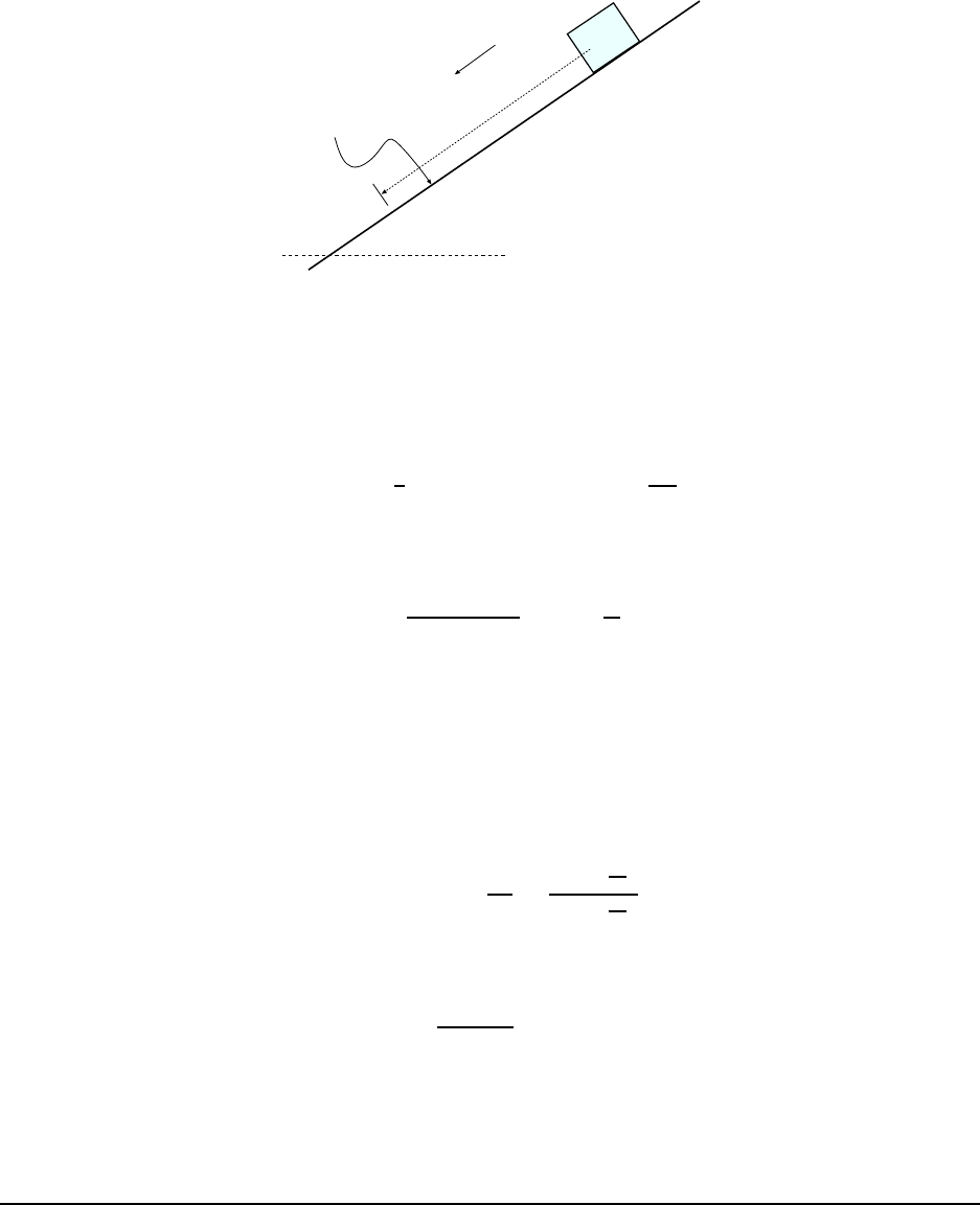
78 CHAPTER 5. FORCES II
40
o
0.800 m
Rough!
x
Figure 5.8: Block slides down rough inclined plane in Example 3.
the block we can find its acceleration; with the x axis pointed down the slope (as we often
do in these proble ms), with v
0x
= 0 we have:
x = 0 +
1
2
a
x
t
2
=⇒ a =
2x
t
2
Plug in the numbers and get a
x
:
a =
2(0.800 m)
(0.600 s)
2
= 4.44
m
s
2
We’ve solved the general problem of a block sliding down a rough inclined plane; In
Eq. 5.6 we found:
a
x
= g sin θ −µ
k
g cos θ = g(sin θ − µ
k
cos θ)
where θ is the angle of the incline. Since µ
k
is the only thing we don’t know here, we can do
some algebra and solve for it:
sin 40
◦
− µ
k
cos 40
◦
=
a
x
g
=
(4.44
m
s
2
)
(9.80
m
s
2
)
= 0.454
µ
k
cos 40
◦
= sin 40
◦
− 0.454 = 0.189
µ
k
=
(0.189)
cos 40
◦
= 0.247
So we get a coefficient of friction of 0.247 for the block sliding on the surface.
5.2 .2 Uniform Circular Motion
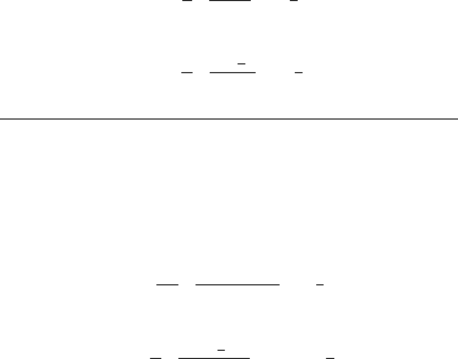
5.2. WORKED EXAMPLES 79
4. A small mass moves on a circular path of radius 2.50 m with constant speed; it
makes one revolution every 3.20 s. (a) What is the speed of the mass? (b) What
is the magnitude of its centripetal acceleration?
(a) Every time the mass moves around the circle, it travels a distance
C = 2πr = 2π(2.50 m) = 15.7 m
This happens in a time T = 3.20 s so the speed of the mass must be
v =
C
T
=
(15.7 m)
(3.20 s)
= 4.91
m
s
From Eq. 5.8 the centripetal acceleration has magnitude
a
c
=
v
2
r
=
(4.91
m
s
)
2
(2.50 m)
= 9.64
m
s
2
5. Find the centripetal acceleration of a point on the equator of the Eart h due
to the rotation of the Earth about its axis [Ser7 7-15a]
A point on the Earth’s e quator moves in a circle of radius
R
earth
= 6.38 × 10
6
m
and the period of T = 1 day = 86400 s. So the spe ed of that point is
v =
2πR
T
=
2π(6.38 × 10
6
m)
(86400 s)
= 464
m
s
Then from Eq. 5.8 the centripetal accelerati on of this point has magnitude
a
c
=
v
2
R
=
(464
m
s
)
2
(6.38 ×10
6
m)
= 3.37 × 10
−2
m
s
2
(The direction of its acceleration is toward the center of the Earth, i.e. downward.)
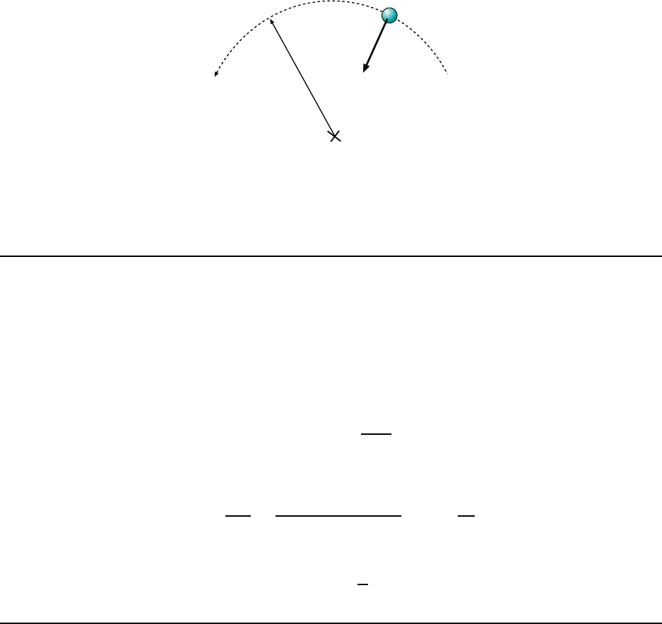
80 CHAPTER 5. FORCES II
0.25 m
F
c
Figure 5.9: Ball moves in a circular arc.
5.2 .3 Circular Motion and Force
6. A 0.015 kg ball is shot from t he plunger of a pinball machine. Because of a
centripetal force of 0.028 N, the ball follows a circular arc whose radius is 0.25 m.
What is the speed of the ball? [CJ6 5-11]
A picture of the ball moving on its circular path is given in Fig. 5.9. The ball moves in
a circular path because the net force on the ball points toward the center of the circle and
has magnitude
F
net
= F
c
=
mv
2
r
Since we are given F
c
, m and r, we can solve for v:
v
2
=
F
c
r
m
=
(0.028 N)(0.25 m)
(0.015 kg)
= 0.47
m
2
s
2
So then
v = 0.68
m
s
7. A 200 g block on a 50 cm–long str ing swings in a circle on a horizontal fri ction-
less table at 75 rpm. (a) What is the speed of the block? (b) What is the tension
in the string? [KJF 6-14]
(a) The motion of the block is shown in Fig. 5.10. We are given the number of revolutions
the block makes in one minute; how do we get the speed for that? We note that i n each
revolution the block travels a distance
C = 2πr = 2π(0.50 m) = 3.14 m
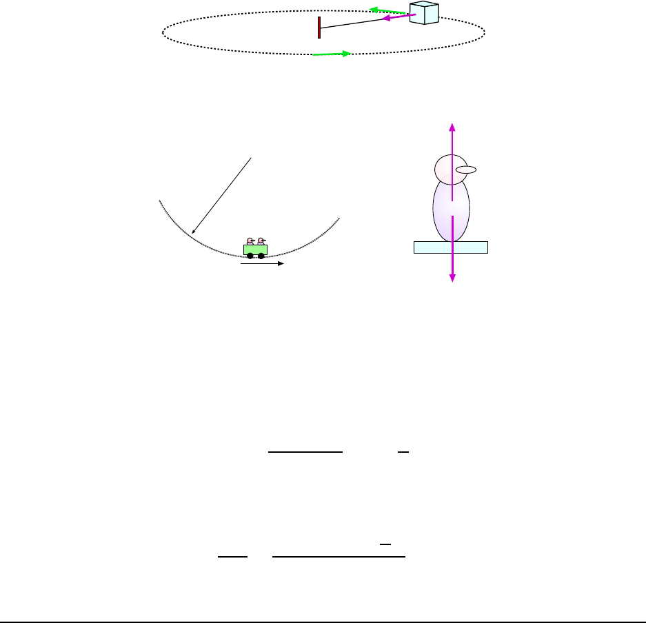
5.2. WORKED EXAMPLES 81
v
v
50 cm
T
Figure 5.10: Block swings in a circular horizontal path.
30 m
v
mg
F
seat
(a)
(b)
Figure 5.11: (a) Roller coaster with passengers at a dip. (b) The forces acting on a passenger at the
bottom of the dip.
and if the block travels 75 times this distance in minute its speed must be
v =
75(3.14 m)
60.0 s
= 3.92
m
s
(b) There is only one force acting on the block, namely that of the string tension and it
pulls inward. The net force on the block must be F
c
= mv
2
/r (inward) so that gives us
T =
mv
2
r
=
(0.200 kg)(3.92
m
s
)
2
(0.50 m)
= 6.2 N
The tension in the string is 6.2 N.
8. The passenge rs in a roller coaste r feel 50% heavier then their true weight as
the car goes through a dip with a 30 m radius of curvature. What is the car’s
speed at the bottom of the dip? [KJF6-19]
Whoa! Passengers feel heavier? Speed at the bottom of the dip? Huh?
The motion of the car with its passengers i s shown in Fig. 5.11(a). We don’t know the
speed v but we do know that since the car and its c ontents has a speed v and is in circ ular
motion where the radius of the motion is 30 m. So the acceleration of the car is toward
82 CHAPTER 5. FORCES II
the center of the circle, that is to say, upward and has magnitude a
c
= v
2
/r. (Here we
assume that the only forces on the car and passengers are vertical; there is no tangential
acceleration) So the acceleration of any one of the passengers a lso has magnitude v
2
/r and
is directed upward.
So if the mass of a passenger is m then the net force on that passenger must have
magnitude mv
2
/r and be directed upward.
The forces acting on a passenger are shown in Fig. 5.11(b). There is the force of gravity,
mg, downward and also the force of the seat, F
seat
, which is directed upward. These forces
do not have equal magnitude because as we just said, the net force has magnitude
mv
2
r
and
is directed upward. So using our force diagram, Newton’s 2nd law gives
F
seat
− mg =
mv
2
r
But the problem tells something about F
seat
. Normally when we sit in chairs we are not
accelerating; then the chair’s force is equal to that of gravity (the weight): F
seat
= mg. We
feel this force of the chair. For t he passengers i n the car F
seat
is l arger; the problem tells us
that the seat’s force is 50% larger than that of gravity:
F
seat
= (1.50)F
grav
= 1.50mg
and using this fact in the first equation gives
(1.50)mg − mg = (0.50)mg =
mv
2
r
which gives (cancel the m):
v
2
= (0.50)gr = (0.50)(9.80
m
s
2
)(30 m) = 147
m
2
s
2
and the n
v = 12
m
s
9. In the Bohr model of the hydrogen atom, an electron (mass m = 9. 11×10
−31
kg)
orbits a proton at a distance of 5.3 × 10
−11
m. The proton pulls on the electron
with an electric forc e of 8.2 ×10
−8
N. How many revolutions per second does the
electron make? [KJF 6- 38]
A picture of this model for the hydrogen atom is shown in Fig. 5.12. The electron orbits
in a circular orbit of radius r with speed v. The only force on the electron is the electrical
force which points inward and has magnitude
F
c
= F
elec
=
mv
2
r
= 8.2 × 10
−8
N
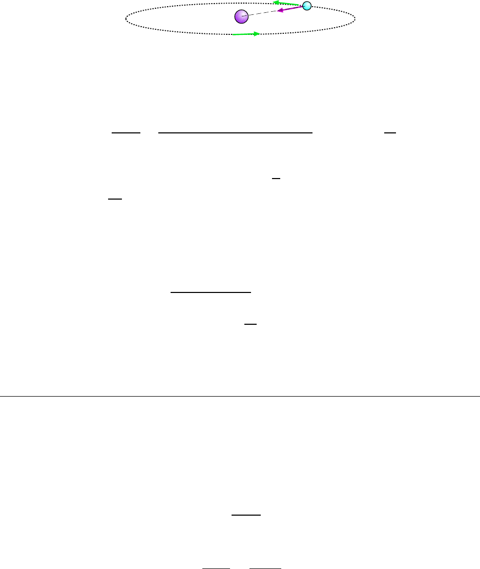
5.2. WORKED EXAMPLES 83
v
v
F
elec
r
proton
electron
Figure 5.12: Electron orbits the proton in the Bohr model.
From this we can solve for the speed v:
v
2
=
rF
elec
m
=
(5.3 × 10
−11
m)(8.2 × 10
−8
N)
(9.11 × 10
−31
kg)
= 4.8 × 10
12
m
2
s
2
so then
v = 2.2 × 10
6
m
s
This speed is ab out
1
100
of the speed of light.
In one second the electron will travel 2.2 × 10
6
m, but the distance covered i n one revo-
lution is
C = 2πr = 3.3 × 10
−10
m
so that the number of revolutions made in one second is
N =
(2.2 × 10
6
m)
(3.3 × 10
−10
m)
= 6.7 × 10
15
rev
so the orbital rate of the electron is 6.7 ×10
15
rev
s
. This is a large number, but the situation
(motion of an electron inside an atom) is rather exotic!
5.2 .4 Orbital Motion
10. One of the moons of Jupiter (Europa) orbits Jupiter in a (roughly) circular
orbit with a radius of 670, 900 km. The period of the orbit is 3.55 days. From this
information, what is the mass of Jupiter?
Eventually we will use Eq. 5.11 here to get m
1
from r and T , but first we need to get
things in the r ight uni ts. In meters, the radius of the orbit r is
r = (670, 900 km)
10
3
m
1 km
!
= 6.71 ×10
8
m
and the period is
T = (3.55 day)
24 hr
1 day
!
3600 s
1 hr
= 3.07 × 10
5
s
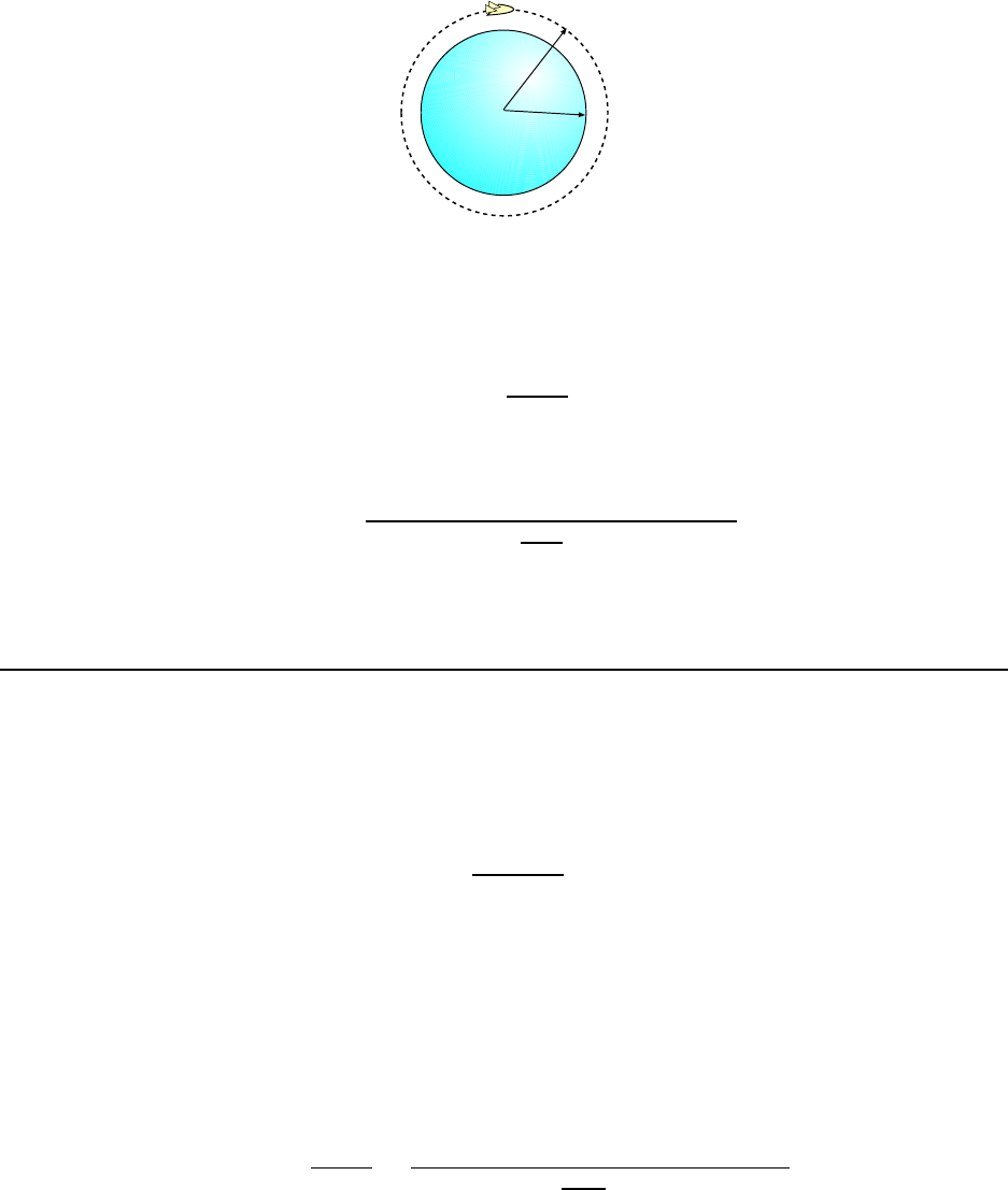
84 CHAPTER 5. FORCES II
r
R
Figure 5.13: Space shuttle in orbit around the earth.
Doing some algebra on Eq. 5.11 to isolate the mass of the central body m
1
gives:
m
1
=
4π
2
r
3
GT
2
and plugging in the numbers (use the form of G in Eq. 4.4) gives:
m
1
=
4π
2
(6.71 × 10
8
m)
3
6.67 × 10
−11
m
3
kg·s
2
(3.07 × 10
5
s)
2
= 1.90 × 10
27
kg
We find that the mass of Jupiter is 1.90 × 10
27
kg.
11. The space shuttle is in a 250−mile-high orbi t. What are the shuttle’s orbital
period (in minutes) and its speed? [KJF 6- 33]
We diagram the problem, as in Fig. 5.13. We need to convert 250 mi to m:
250 mi = (250 mi)
10
3
m
0.621 mi
!
= 4.03 × 10
5
m
but to find the radius of the shuttle’s orbit (that is, its distance from the center of the earth)
we must add this to the radius of the earth. Thus:
r = R + 4.03 × 10
5
m = 6.37 × 10
6
m + 4.03 × 10
5
m = 6. 77 × 10
6
m
Having the radius of the orbit, and knowing the mass of the earth, we can use Eq. 5.11
to get the period of the orbit:
T
2
=
4π
2
r
3
Gm
1
=
4π
2
(6.77 × 10
6
m)
3
(6.67 × 10
−11
N·m
2
kg
2
)(5.98 ×10
24
kg)
= 3.17 × 10
7
s
2

5.2. WORKED EXAMPLES 85
Then:
T = 5.54 × 10
3
s
1 min
60 s
= 92.3 min
We can get the speed of the shuttle using Eq. 5.7:
v =
2πr
T
=
2π(6.77 × 10
6
m)
(5.54 × 10
3
s)
= 7.68 × 10
3
m
s
86 CHAPTER 5. FORCES II
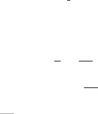
Chapter 6
Energy
6.1 The Important Stuff
6.1 .1 Introduction
While Newton’s laws form the basis of physics, experience has shown that we need some other
concepts and laws to be able to deal with problems effectively. The present chapter and the
next one deal with some new quantities and the rule s which they obey. The quantities are
energy and mome ntum.
6.1 .2 Kinetic Energy
We make a definition of a quantity which we will soon find to be quite useful. For a particle
of mass m moving at speed v, the kinetic energy of the particle is defined by:
KE =
1
2
mv
2
(6.1)
What sort of q uantity is this? It is a scalar , that is, it is s single number which does not have
any direction associated with it (unlike velocity which is a vector). It is always a positive
number since m and v
2
are always positive.
The units of this quantity have to be those of mass multiplied by those of speed squared,
that is,
kg ·
m
s
2
=
kg·m
2
s
2
This is a new and im portant combination which is called the joule. Thus:
1 joule = 1 J = 1
kg·m
2
s
2
(6.2)
Other units of energy sometim es see n are:
1 erg = 1
g·cm
2
s
2
= 10
−7
J and 1 MeV = 1.602 × 10
−19
J
87
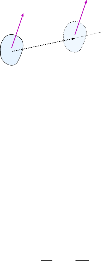
88 CHAPTER 6. ENERGY
F
s
F
q
q
Figure 6.1: Constant force F acts on an obj ect as it is displaced by s. Work done is F s cos θ.
The erg is the unit of energy in the cgs system of units; the MeV is encountered when we
deal with atomic processes.
6.1 .3 Wo rk
We have one more quantity to define before we say anything of any substance. The quantity
is work. When a force acts on an object which undergoes a displacement (i.e. it moves)
then work is done.
We first consider a speci al case for computing work. This is where the force F is constant
(keeps the same magnitude and direction) and where t he displacement of the mass is along
a straight line; so the displacement (change in location r) is some vector s; see Fig.6.1
Finally, suppose the angle between the force vector F and the displacement s is θ. Then
the work done by t his f orce is
W = F s cos θ (6.3)
We have several things to discuss ab out de finition 6.3 before discussing why it’s impor-
tant.
First off, work is a scalar meaning that it is a single number. The units of work are t hose
of force times those of distance (a cosine has no units) which is the c ombination:
N · m =
kg·m
s
2
· m =
kg·m
2
s
2
which you’ll notice is the very same combination that made up the units for kinetic ene r gy,
the combination that we called a “joule”. Thus, work is measured in joules.
Next we note that while F and s are both positive, the cosine of an angle can b e negative
(as the n the angle is between 90
◦
and 180
◦
) so that work (W ) can be negative.
Finally there are three special c ases for θ that we will want to keep in mind: When
the force acts in the same direction as the displacement then θ is zero, cos θ = 1 and then
W = F s. When the force acts i n the opposite direction as the displacement then θ = 180
◦
,
cos θ = −1 and then W = −F s. When the force acts in a direction perpendicular to that

6.1. THE IMPORTANT STUFF 89
of the displ acement then θ = 90
◦
, cos θ = 0 and the work done is zero. A force acting
perpendicular to the di rection of motion does no work.
Finally, it will be of use to find the total work done by all the forces acting on a mass.
To get this, we simply add up the work done by each individual force. One can also find the
net force acting on the mass and find the work done by it; the result is the same.
6.1 .4 The Work–Energy Theorem
What are these definitions good for? One can show that the quantities kinetic energy (KE)
and work (W ) are related. If we consider the motion of a particle over a certain time interval
we can consider the total work done on the particle, W
tot
. We can also consider its change
in kinetic energy, which is just
∆KE = KE
f
− KE
i
=
1
2
mv
2
2
−
1
2
m
2
1
The work energy theorem tells us that they are the same:
W
tot
= ∆KE (6.4)
6.1 .5 Potential Energy
Some physics problems can be done using the Work–Energy Theorem but in general we
need some further definitions and theorems so that it becomes really useful. In particular,
calcul ating the work done by the various forces can be made much simpler.
One can show that when an object of mass m moves from a he ight y
1
to a height y
2
, then
work done by grav ity is
W
grav
= −mg(y
f
− y
i
) = −mg∆y . (6.5)
This is an interesting result because W
grav
depends only on the difference in heights between
the i nitial and final positions. The path that t he particle took between the two places does
not matter! The work done is just a difference in the quantity −mgy evaluated between the
initial and final locations.
We will see some other forces for which the work done i s also expressible as a difference
in some expression between the final and initial positions. Not all forces have this property
but some of the more interesting ones do. Such forces are called conservative forces and
for these forces it is easiest to find and use the expression whose difference gives W .
To be precise, it’s the negative of the difference in some quantity which we want to equal
W ; the quantity is called the potential energy, PE. Thus, for forces which p ermit us to
have a simple expression for the work, we define:
∆PE = −W (6.6)
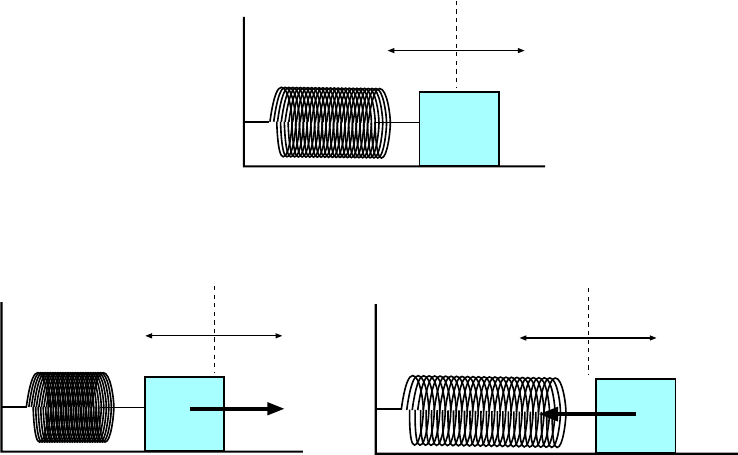
90 CHAPTER 6. ENERGY
x
0
x
0
x
0
F
F
F = 0
(a)
(b)
(c)
Figure 6.2: Spring exerts a f orce on the block which opposes the displacement of the block from the
equilibrium positi on. (a) Spring has its natural length; no force. (b) Spring is compressed; force goes
outward. (c) Spring is stretched; force goes inward.
Comparing this with Eq. 6.5, the potential ener gy for the gravity force (near the surface
of the earth) is
PE
grav
= mgy (6.7)
where y is the usual vertical coordinate.
As mentioned, not all forces are conservative. The k inetic friction force does not have
this property. As you might expect, such forces are called nonconservative.
6.1 .6 The Spring Force
In order to have some variety at this point, I wil l introduce another kind of force which is
important in physics. This is the force exerted by an ideal spring on something attached to
its end.
In Fig. 6.2 we show the basic behavior of a spring. When it is unstretched or uncompressed
it has an equilibrium length. In that case there is no force exerted on the block which is
attached to one end. When it is compressed (as in (b)) or stretched (as in (c) ) then a force is
exerted on the block; the direction of the force is o pposite the direction of the displacement.
Also, the spring force has a greater ma gnitude the more we c ompress or stretch the spring
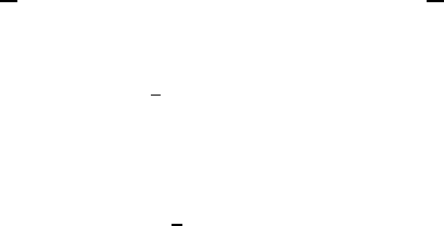
6.1. THE IMPORTANT STUFF 91
(i.e. as |x| gets bigger). For the “ide al spring”, the magnitude of the force is proportional to
the amount of compression or stretch of the spring away from the equilibrium position. If we
consider the motion of the mass along the x axis and if x = 0 corresponds to the equilibrium
position then the force of the spring is given by:
F
x
= −kx (6.8)
where the number k is a constant and depends on the stiffness of the spring. (It is positive;
the minus sign in Eq. 6.8 makes F
x
opposite in sign to t he displacement x.) It is called
the force c onstant of the spring and since it is equal to |F/x|, its units are those of force
divi ded by those of distance, or
N
m
. (This combination is also equal to
k
s
2
.)
One can show that if the mass on the end of the spring goes from x
1
to x
2
, the work done
by the spring force is
W
spring
= −
1
2
k(x
2
2
−x
2
1
)
which is true regardless of how the mass gets from x
1
to x
2
. Then Eq. 6.6 gi ves us the
expression for the potential energy of the spring force:
PE
spr
=
1
2
kx
2
(6.9)
6.1 .7 The Principle of Energy Conservation
Now we show why the idea of potential energy is useful.
The forces in nature are either conservative or non-conservative; when we compute the
total work done by all the forces we can separate the sum into two parts, one due to the
conservative forces and one due to the non-conservative forces:
W
total
= W
con s
+ W
non−cons
putting this into Eq. 6.4 we have:
W
total
= W
con s
+ W
non−cons
= ∆KE
Now we note from Eq. 6.6 the work by the conservative forces is equal to the change in all
the kinds of potential e nergy:
W
con s
= −∆PE
Putting this into the previous equation,
−∆PE + W
non−cons
= ∆KE
And then a little rearranging gives:
∆PE + ∆KE = ∆(PE + KE) = W
non−cons

92 CHAPTER 6. ENERGY
One more definition and we’re done. We define the total energy E to be the sum of
the potential and kinetic e nergies:
E = PE + KE (6.10)
and the n the last equation become s:
∆E = ∆ ( PE + KE) = W
non−cons
(6.11)
In words, the change in the total energy of a system equals the work done by the non-
conservative forces.
Oftentimes we have a situation where there are no non-conservative forces; for ex ample
if there are no friction force that need be considered. In that case, W
non−cons
is zero and
Eq. 6.11 reduces to
∆E = E
f
− E
i
= 0 (No non-conservative forces! ) (6.12)
which tel ls us t hat for this case the total energy does not change. When a quantity in
physics remains the same in spite of other changes in the system we say that the quantity
is conserved. So we would also say that in the absence of non-conservative forces, total
energy is conserved.
6.1 .8 Solving Problems With Energy Conservation
The principle of energy conservation can be useful in solving physics problems where the
motion of a particle is complicated but the kinds of forces involved are simple, and also if
you aren’t being asked for a time interval—because time does not enter into our equations
for energy.
In the cases where there are no friction f orces (or any other forces which do work) we can
use Eq. 6.12. If we setup expre ssions for the t otal energy of a system before and after some
motion takes place (and set them equal) we may be able to solve for some unknown speed
or distance.
If the problem does involve a friction force or some other force which does work we would
have to use the more general Eq. 6.11 but it too can be useful i f we have some way of treating
the non–coservative force.
6.1 .9 Power
One more concept involving work and energy is useful in studying the world. We’ve discussed
how one calculates work done by a force. This quantity involved force and distance but it
did not involve time. If an amount of work W is done in a time t we define the average
power from thi s force as
P =
W
t
(6.13)

6.2. WORKED EXAMPLES 93
Power is the expression of how rapidly energy is transferre d from one system to another.
Like work and energy, power is a scalar and its uni t s are those of energy (joules) divided
by those of time (seconds). We call the combination
J
s
a watt:
1 watt = 1 W = 1
J
s
= 1
kg·m
2
s
3
If we consider very sm all time intervals t in Eq. 6.13 we find the instantaneous power P
from the force.
In the speci al case of a particle moving in one dimension, acted on by a constant force
along this direction and moving with instantaneous veloc ity v
x
, we can find the instantaneous
power from:
P = F
x
v
x
(6.14)
6.2 Worked Examples
6.2 .1 Kinetic Energy
1. At what speed does a 1000 kg compact car have the same k inetic ener gy as a
20, 000 kg truck going at 25 km/hr? [KJF 10-8]
Let m and v be the mass and speed of the compact car and M and V be the mass and
speed of the truck. We don’t know v but we have the condition that the kinet ic energies of
the two are equal. Thus:
1
2
mv
2
=
1
2
MV
2
=⇒ v
2
=
MV
2
m
=
(2.00 × 10
4
kg)(25
km
hr
)
2
(1.00 × 10
3
kg)
Solving this for v gives
v = 112
km
hr
6.2 .2 The Spring Force
2. An ideal spring has a force constant of 820
N
m
. How far should one deform i t
from its equilibrium le ngth so that 0.100 J of energy is stored?
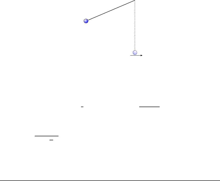
94 CHAPTER 6. ENERGY
60
o
v
1.20 kg
2.00 m
Figure 6.3: Mass on the end of a string is pulled back by 60
◦
and then released. When the mass reaches
the lowest point, what is the tension in the string?
Use Eq. 6.9 and solve for x:
PE
spr
=
1
2
kx
2
=⇒ x
2
=
2(PE
spr
)
k
Plug in the numbers:
x
2
=
2(0.100 J)
(820
N
m
)
= 2.44 × 10
−4
m
2
=⇒ x = 1.6 ×10
−2
m = 1.6 cm
We ne ed to compress the spring by 1.6 cm.
6.2 .3 Solving Problems With Energy Conservation
3. A smal l 1.20 kg mass is attached to the end of a string of length 2.00 m; the
string is pulled back by 60.0
◦
from the vertical, as shown in Fig. 6.3. T he mass
is released and it swings downward on the string. If t he string breaks under a
tension of more than 20 N, will the mass be able to get t o the bottom of its swing
as shown in the figure?
For reasons that we’ll see as we work the problem, the maximum tension in the string
will oc cur at the bottom of the swing so if the string ever breaks it will break then. So we
will assume it gets to the bottom and then calculate the string tension at that point.
The string tension at the bottom is not equal to the weight of the mass. We have to
analyze the forces and apply Newton’s 2nd law!
The forces acti ng on the mass at the bottom of the swing are shown in Fig. 6.4. They
are gravity, mg downward and the string tension T upward. These forces do not add to zero
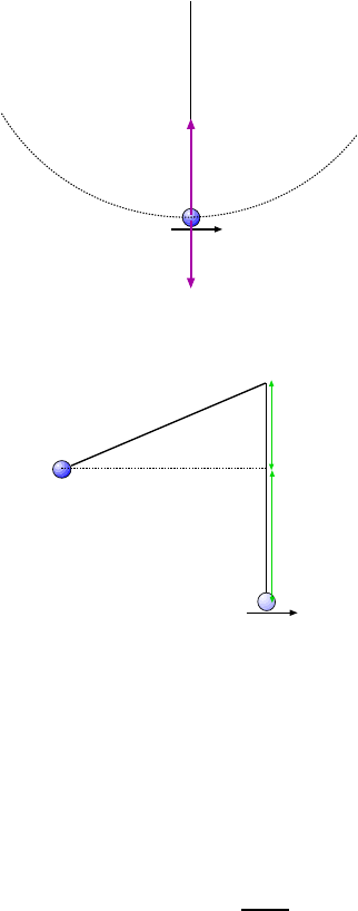
6.2. WORKED EXAMPLES 95
v
m = 1.20 kg
R = 2.00 m
mg
T
Figure 6.4: Forces acting on the mass at the bottom of the swing.
q = 60
o
v
R = 2.00 m
Rcosq
R - Rcosq
Figure 6.5: Some geometry for Example 3.
because at this point the mass is accelerating. How so? The mass is moving on the arc
of a circle of r adius R with speed v and so the radial (inward) forces must add to give the
centripetal force, F
c
= mv
2
/R. Thus:
T − mg =
mv
2
R
(6.15)
where R i s the string length, R = 2.0 m. To find T we will need to k now the speed v at the
bottom of the swing.
We can get v using the conservation of energy. There are no friction forces here , only the
conservative force of gravity and the string tension T which does no work because it always
pulls perpendicularly to the motion of the mass. So total mechanical energy is conserved,
E
i
= E
f
.
Taking the bottom of the swing to be “zero height” a little geometry (see Fig. 6.5) show
that the init ial height of the mass was
y
i
= R − R cos θ = R(1 − cos θ) = (2.00 m)(1 − cos 60
◦
) = 1.00 m
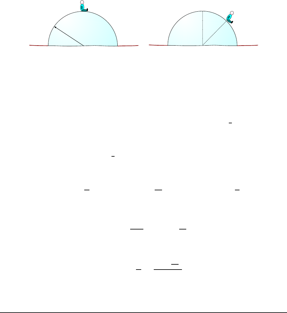
96 CHAPTER 6. ENERGY
R
q
(a)
(b)
Figure 6.6: (a) Boy rests at top of frictionless hemisphere; he starts to slip down one side of it! (b) At
some angle θ from the vertical he loses contact with the surface.
So energy conservation gives
PE
i
+ KE
i
= PE
f
+ KE
f
=⇒ mgy
i
+ 0 = mgy
f
+
1
2
mv
2
Here cancel a factor of m and do some algebra:
g(y
i
− y
f
) =
1
2
v
2
=⇒ v
2
= 2g(y
i
− y
f
)
Plug in the numbers and get
v
2
= 2(9.80
m
s
2
)(1.00 m − 0) = 1.96
m
2
s
2
=⇒ v = 4.43
m
s
Now we have the value of v
2
that we can use in Eq. 6.15. Some algebra on that equation
gives
T = mg +
mv
2
R
= m
g +
v
2
R
!
Now plug in the numbers and get
T = (1.20 kg)
(9.80
m
s
2
) +
(19.6
m
2
s
2
)
(2.00 m)
= 23.5 N
But the string cannot support a tension this large! So the string will break before the mass
gets to the bottom of the swing.
4. A small boy sits at the top of a frictionless hemisphere of radius R, as shown
in Fig. 6.6(a). He starts to slip down one side of it and at some angle θ measured
from the vertical he loses contact with the surface, as shown in Fi g. 6.6(b). Find
the angle θ.
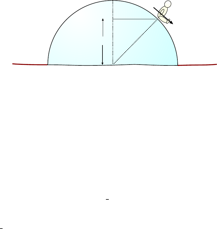
6.2. WORKED EXAMPLES 97
q
v
R
Rcosq
Figure 6.7: Boy at position given by θ has sp eed v and height R cos θ
This is a classic and somewhat challenging problem but it does not r equire any more
math than simple trig.
We focus on the point at which the loss of contact occurs. While the boy starts from
rest at the top of the sphere, his spe ed is v at this point. As mentioned, his position is given
by the angle θ as m easured form the vertical so that while his initial height was R it is now
R cos θ; se e Fig. 6.7.
Since there are no friction forces acting, the boy’s total energy is conserved between the
initial position at the top and the final position at θ, that is:
KE
i
+ PE
i
= KE
f
+ PE
f
Using PE = mgy this is
0 + mgR =
1
2
mv
2
+ mgR cos θ
where m is the mass of the b oy. Do a little algebra on this and get:
1
2
mv
2
= mgR − mgR cos θ = mgR(1 − cos θ) =⇒ v
2
= 2gR(1 − cos θ )
The condition that the boy “loses contact” with the surface means that there is no normal
force from the surface on the boy at some point. We know that the surface exerts no sideways
(tangential) force on the boy because the r e is no friction. But in gene r al t he surface can
push outward on the boy with some force F
N
. (It cannot pull inward, and that is why the
boy will fly off at some point.)
The forces on the boy when he is at position θ are shown in Fig. 6.8. Gravity mg pulls
downward and the normal force F
N
pushes outward. The force of gravity has been spli t into
components: Doing a little geome t ry, we can see t hat a component mg cos θ points inward
toward the center of the sphere and a component mg sin θ points tangentially.
Now at the moment the boy loses contact he is following the path of a circl e (with speed
v) so that the net force in the inward direction is the centripetal force, mv
2
/R. (It is true
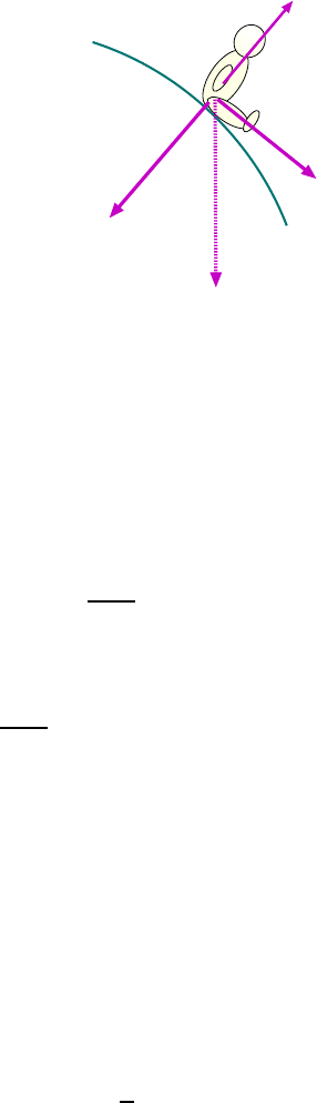
98 CHAPTER 6. ENERGY
mg
mgsinq
mgcosq
q
F
N
Figure 6.8: Forces on the boy at position given by θ .
that there is also a tangential force but that doesn’t matter.) According to our force diagram
the net force in the inward direction is
F
c
= mg cos θ − F
N
and so
mv
2
R
= mg cos θ − F
N
.
But at the moment he l oses contact, F
N
= 0 so we get
mv
2
R
= mg cos θ =⇒ v
2
= Rg cos θ
Comparing our results for energy conservation and the centripetal force, we got two
expressions for v
2
. If we equate them, we get
2gR(1 − cos θ) = Rg cos θ
Cancel the Rg and do some algebra:
2(1 − cos θ) = cos θ =⇒ 2 = 3 cos θ
Finally,
cos θ =
2
3
=⇒ θ = 48.2
◦

Chapter 7
Momentum
7.1 The Important Stuff
7.1 .1 Momentum; Systems of Particles
Again we begin the chapter with a definition; later, we’ll see why it’s useful and then use a
new principle to solve problems in physics.
When a particle of mass m has velocity v, its momentum (or more specifically, its
linear momentum), p is defined as:
p = mv (7.1)
That is, momentum is just mass times velocity.
Momentum is a vector, and Eq. 7.1 means that
p
x
= mv
x
p
y
= mv
y
p
z
= mv
z
The units of momentum are those of mass (kg) times those of velocity (
m
s
), that is,
they are
kg·m
s
. Oddly enough people haven’t been able to agree on a special name f or this
combination so we leave it as it is.
7.1 .2 Relation to Force; Impulse
Using Newton’s 2nd law we see how momentum is related to force. Considering forces and
motion in one dimension, if a constant force F
x
acts on a mass m for a time interval ∆t then
F
x
∆t = (ma
x
)∆t = m(a
x
∆t) = m∆v
x
But since
m∆v
x
= m(v
fx
− v
ix
) = mv
fx
− mv
ix
= ∆p
x
99

100 CHAPTER 7. MOMENTUM
then combining the two equations gives
F
x
∆t = ∆p
x
Or, dividing by ∆t,
F
x
=
∆p
x
∆t
(7.2)
so that the f orce on a particle is equal to the rate of change of its momentum.
Eq. 7.2 gives us a definition for the average force acting on a particle. If, during a
time interval ∆t the change in momentum of a particle is ∆p, then the average f orce on the
particle for that period is
F =
∆p
∆t
(7.3)
People often make a definition to deal with the change in momentum of a particle. If
over a certai n time interval a particle has a change i n momentum ∆p, they say that the
impulse, I imparted to the particl e is
I = ∆p (7.4)
From this, we see that impulse is a vector with the same uni t s as momentum.
Since from Eq. 7.3 we have F∆t = ∆ p, from the definition of impulse we also have
F∆t = I
7.1 .3 The Principle of Momentum Conservation
Oftentimes in physics we are faced wi th the problem of two objects which are moving along
free from forces; the objects interact with each other and then move apart, again free from
outside forces, as shown in Fig.7.1. Often we want to call such an event a “collision”. The
velocities (both magnitude and direction) of the masses after the event can be quite different
from what they were before the event.
The problem with the analysi s of such an event is that the force between the two objects
may not be known very well. Generally when objects collide this force is very strong, very
brief and very complicated. In such a situation does physics have anything at all to say
about the collision?
Here I’d like to give a simple derivation of the principle of mome ntum conservation
because the math is simple and it’s important to understand the basic reason behind this
princi ple.
Consider what happens duri ng the interaction between A and B in Fig. 7.1(b). They
exert forces on each other, but from Newton’s 3rd law these forces are equal and opposite:
F
B on A
= −F
A on B
(7.5)

7.1. THE IMPORTANT STUFF 101
(a)
(b)
(c)
A
B
A
B
A
B
v
Bf
v
Af
v
Bi
v
Ai
Figure 7.1: A colli sion between masses A and B. (a) Ma sses move freely with velocities v
Ai
and v
Bi
. (b)
For a brief time the masses exert a force on one another. The force changes their velocities. (c) The masses
move freely again, with velocities v
Af
and v
Bf
Consider a very small time interval ∆t during the interaction over which we can take force
as being constant. Multiply both sides of Eq. 7.5 by ∆t and get:
(F
B on A
)∆t = −(F
A on B
)∆t (7.6)
Now we’re assuming that B is the only thing exerting a force on A and vice versa. That
means that F
B on A
∆t gives the change in momentum of A, ∆p
A
over this time interval ∆t .
Similar remarks hold for B so we can write:
(∆p
A
)
interval ∆t
= −(∆p
B
)
interval ∆t
(7.7)
So the changes in momentum for A and B are equal and opposite over every little bit of the
interaction. If we add up the changes in momentum over all little bits of the interaction we
still find that they are equal and opposite for the whole interaction period :
(∆p
A
)
whole
= −(∆p
B
)
whole
(7.8)
Now write the changes in momentum in terms of the mome nta before and after the
interaction:
p
Af
− p
Ai
= −(p
Bf
−p
Bi
) (7.9)
A little rearranging gives:
p
Ai
+ p
Bi
= (p
Af
+ p
Bf
) (7.10)
Now a definition. We’ll let P stand for the total momentum of all the particles,
P = p
A
+ p
B
(7.11)
102 CHAPTER 7. MOMENTUM
With this definition, then the left side of 7.10 is the initi al value of P and the right side is
the final value of P. So we have:
P
i
= P
f
(7.12)
that is, the value of the total momentum stay s the same, or as we say in physics, is conserved.
We need to recall the conditions under which we could make t his statement (our assump-
tions): We assumed that during the interaction, A and B were interacting with each other
but felt no forces from anything else. Another way to say this is that during the interaction,
the two objects were isolated; bec ause of that, their total momentum was conserved.
The principle can be made more general by includi ng more particles, and the lesson can
be stated as:
For a system of i solated particles, the total momentum is conserved.
7.1 .4 Collisi ons; Problems Using the Conservation of Momentum
Sometimes we are faced with a problem where there are two or interacting particles which
“feel” no forces from anything else, i.e. they are isolated. Sometimes we have a situation
where we are consideri ng the m otion of several particles over such a short period of time
that we can safely ignore the external forces but we can’t ignore the forces between the
particles. Then, for the purposes of the problem, the particles are (again) “isolated”. The
forces between t he particles may be very complicated, but that doesn’t matter. The total
momentum of the particles will stay the same before and after the interaction.
Examples of where such an interaction can occur are:
• When two particles travel freely, bounce off one another and then travel away from one
another in new directions; this is what we normally think of as a “collision”.
• When two particl es come together and stick to one another; the combined mass travels off
as one unit (with a mass equal to the sum of the individual masses).
• When a single mass explodes and the individual parts fly off in different dire ctions; we
would call this an “explosion”. Again, the sum of all the masses is the same be fore and after.
Though total momentum stays the same during these processes, what about the energy
of the particles? More specifically, since in the r apid interactions we are considering the
potential energy of the system doesn’t change by much we ask what happens to the kinetic
energy of the particles.
In general, the total kinetic energy can remain the same or decrease or even increase
for a collision; it depends on the nature of the interacting objects and the kind of force
the exe r t on each other. The usual case is that when real objec t s collide the force is i n
small part frictional in nature and then kinetic energy is lost, or rather it changes form to
thermal energy. But it is possible that the impact releases chemical or other stored energy
from an exploding element and then the kinetic energy would increase. But if the surfaces
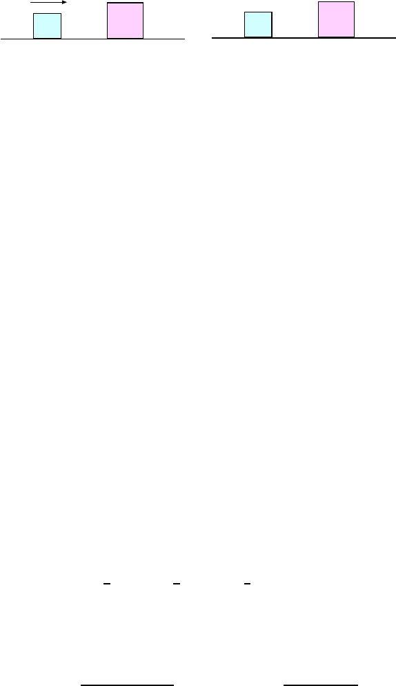
7.1. THE IMPORTANT STUFF 103
m
1
m
2
v
1i
m
1
m
2
v
1f
v
2f
(a)
(b)
v
2i
= 0
Figure 7.2: Elastic collision in one dimension. (a) Mass m
1
has initial velocity v
1i
and mass m
2
is at rest.
(b) Final velocities of the two masses are v
1f
and v
2f
. Fo rmulae for these velocities are given in the text.
of the objects are very tough and springy the change in energy might be so small as to be
unmeasurable.
When t he total kinetic energy stays t he same in a c ol lision we say that it is an elastic
collision. If KE is lost (or gained) we say that the collision is inelastic.
A special name is gi ven to the case mentioned above where one particle strikes another
and sti cks. Such a colli sion is called complet ely inelastic.
If we know beforehand that a collision is elastic then we have some additional information
which can help us solve a proble m. As an example we consider a situation which is easy to
set up in the lab: A one-dimensional collisi on in which a mass m
1
is moving toward another
mass m
2
which is at rest. Knowing that the collision is elastic we want to find the velocities
of the masses after the collision.
The problem is diagrammed in Fig.7.2. In the colli sion the r e are no (appreciable) exte r nal
forces, so momentum is conserved:
m
1
v
1i
+ 0 = m
1
v
1f
+ m
2
v
2f
(7.13)
Here the v’s are velocities so that they can be positive or negative. However i f we say that
v
1i
is positive then v
2f
had better be positive; if the second mass went backward after the
collision, both masses would have to be moving backward, which is nonsense! But v
1f
could
possibly be negative; that is the case where m
1
bounces backwards after t he coll ision.
Now if we also know that kinetic energy is conserved in the c ollision then we can write
another equation:
1
2
m
1
v
2
1i
=
1
2
m
1
v
2
1f
+
1
2
m
2
v
2
2f
(7.14)
If we take the masses m
1
and m
2
and v
1i
as “known” and the final velociti es v
1f
and
v
2f
as unknown then the two equations 7.13 and 7.14 all ow us to find the two unknown
velocities. This involves some algebra which I’ll skip, but the solution is:
v
1f
=
(m
1
− m
2
)v
1i
(m
1
+ m
2
)
v
2f
=
2m
1
v
1i
(m
1
+ m
2
)
(7.15)
Eq. 7.15 t ells us some i nteresting things. If the masses are equal (m
1
= m
2
) then the
equations tell us that v
1f
is zero— the first mass stops— and v
2f
= v
1i
, the sec ond mass
moves off with the same velocity that the first mass had.

104 CHAPTER 7. MOMENTUM
If we consider the case where m
2
is enormous compared to m
1
, then in the solution for
v
1f
we c an replace (m
1
− m
2
) by −m
2
and (m
1
+ m
2
) by m
2
, giving
v
1f
=
−m
2
m
2
v
1i
= −v
1i
so that mass m
1
just reverses its motion. In this case, m
2
will move forward very slowly.
The case where m
1
is enormous compared to m
2
is interesting. We find that v
1f
is almost
the same as v
1i
, but for m
2
we find that since (m
1
+ m
2
) is basic al ly the same as m
1
we get
v
2f
≈
2m
1
m
1
v
1i
= 2v
1i
that is, m
2
goes forward with twice the original speed of m
1
. (And m
1
plows ahead with
roughly the same speed.)
7.1 .5 Systems of Particles; The Center of Mass
Newton’s laws as given in Chapter 4 really apply to point masses (“particles”) and yet we’ve
been applying them t o real objects which have non–zero dimensions. Have we b een correct
in doing so? If so, how was it correct?
There are two problems in ignoring the fact that real objects have real sizes. First off, a
real object can change its orientation while staying basically in the same place. We say that
a real object can rotate, and we will deal with simple rotations in the next chapter.
Secondly, if an object has a non-zero size it i s somewhat problematical as to what we
mean by the “location” of the object when discussing its kinematics: When we talk about
the “motion” of the obje ct, what particular point of the object are we talking about? The
“middle” of the object, maybe? What do we m ean by “middle”?
A real object can be treated as a collect ion of a whole lot of point particles and with this
treatment and the use of Newton’s laws (which do apply to points) one can show that we
can keep using Newton’s laws for big things (or systems of parti cles) as long as we make the
following r eplaceme nts:
• For the force F
net
in Newton’s 2nd law, use the total external force acting on all parts of
the object. (The parts of the objec t or set of masses may be exerting forces on each other,
but we don’t need to count those.)
• For the mass m, use the total mass of the object or the total m ass of the system of particle s.
Let’s call the total mass M.
• For the acceleration a, realize that we are now talking about the acceleration of a special
point called the center of mass of the object or system of partic les: a
CM
.
With these replacements in mind, the ex pression of N ewton’s 2nd law (fortunately ) looks
the same:
F
net
= Ma
CM
(7.16)
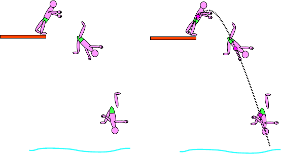
7.1. THE IMPORTANT STUFF 105
(a)
(b)
CM
CM
CM
Figure 7.3: (a) Diver jumps off diving board and does some of that crazy diver-type stuff; action l ooks
very complicated! (b) If we plot the center of mass of the diver, its motion is fairly simple (a parabolic path).
but the terms have new meanings.
With the new usage of Newton’s second law, things which se em to have a complicated
motion have a simpl e aspect. Consider a diver jumping into the water and doing all those
crazy things that divers do, as shown in Fig.7.3. The motion lo oks complicated, but if at
each instant in time we could locate the center of mass of the diver and track its motion, we
would see that it follows a nice parabola as shown in Fig. 7.3(b). Why is that?
The revised version of Newton’s 2nd law says to consider the total (external) force acting
on the diver. Granted, gravity acts on the diver’s various parts but the total force is still
Mg, directed downward. The total mass of the diver is M. So we know that the acceler ation
of the center of mass is simple; it has magnitude Mg/M = g and is directed downward, the
same as for the (point) projectile problem solved back in Chapter 3. There we found that
the general path is a parabola and so that is the shape of the path of the center of mass for
the diver.
7.1 .6 Finding the Center of Mass
So the center of mass has great importance in the physics of a system of particles. How do
we find it?
Here we will just give the formula the center of mass of a set of mass points; for a
continuous mass we use the same principle but it becomes necessary to use calculus. Also
we’ll just work in two dimensions.
If a set of mass p oi nts with masses m
1
, m
2
, m
3
. . . have coordinates (x
1
, y
1
), (x
2
, y
2
),
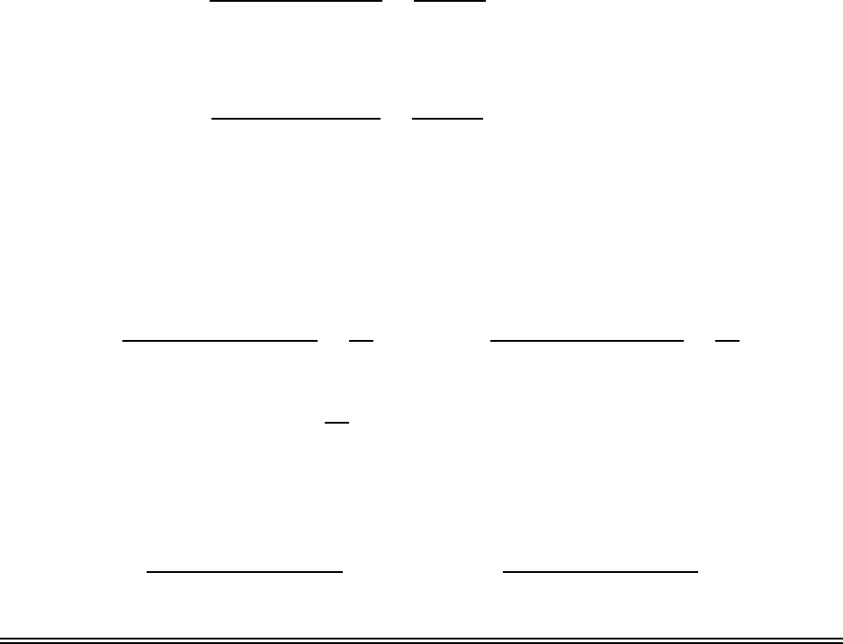
106 CHAPTER 7. MOMENTUM
(x
3
, y
3
). . . then the x coordinate of its center of mass is given by
x
cm
=
m
1
x
1
+ m
2
x
2
+ ···
m
1
+ m
2
+ ···
=
P
i
m
i
x
i
M
with M =
X
i
m
i
(7.17)
Likewise the y coordinate of the center of mass is
y
cm
=
m
1
y
1
+ m
2
y
2
+ ···
m
1
+ m
2
+ ···
=
P
i
m
i
y
i
M
with M =
X
i
m
i
(7.18)
In both cases what we are doing is taking a weighted a verage of the co ordinates of the mass
points, where the “weighting” is done with the ma s ses of the points.
As the members of a set of mass points move around, the location of the ir center of mass
will also move, and it will have its own velocity. The components of the velocity of the center
of mass satisfy an equation similar to that of the location of the cm :
v
cm,x
=
m
1
v
1,x
+ m
2
v
2,x
+ ···
m
1
+ m
2
+ ···
=
P
x
M
v
cm,y
=
m
1
v
1,y
+ m
2
v
2,y
+ ···
m
1
+ m
2
+ ···
=
P
y
M
(7.19)
or:
v
cm
=
P
M
=⇒ P = Mv
cm
. . . which looks like the definition of mome ntum but here it gives the total momentum of a
system of particles.
Finally, the acce leration of the center of m ass satisfies
a
cm,x
=
m
1
a
1,x
+ m
2
a
2,x
+ ···
m
1
+ m
2
+ ···
a
cm,y
=
m
1
a
1,y
+ m
2
a
2,y
+ ···
m
1
+ m
2
+ ···
. (7.20)
7.2 Worked Examples
Chapter 8
Rotational Kinematics
8.1 The Important Stuff
8.1 .1 Rigid Bodies; Ro tating Objects
So far we have had much to say about the motion of obj ects and the way it is determ ined by
the forces acting on those objects. But in all of our examples we were treating the objects
as points (i.e. “particles”), assuming that if they did have any size or internal motion it was
unimportant.
We will now deal with the fact that real objects have a non-zero size and it addition to
the moti on of their center of mass (the translational motion) they can also be in rotation.
We will only deal wi th objects which keep the same shape; the individual bit s of the
object alway s stay at the same distance from one another, i .e. they don’t stretch, compress
or otherwise deform. Such an object is cal led a rigid body and we’ll have enough on our
plate just to deal with such obje cts.
Even after restricting ourselves to rigid bodies, their motion can be very complicated. If
you throw a football the right way it will have a simple kind of rotational motion, as shown
in Fig. 8.1(a). If you throw i t the wrong way it will be rotating in several differe nt ways al l
at once, as in Fig. 8.1(b).
In thi s and the next chapter we will deal with very si mple rotations, usually of the kind
illustrated in Fig. 8.2(a). Here, a r igid body rotates around a fixed axis. Each point of t he
object moves in a c ircle , though the radii of these individual circles will not be the same.
For now, this is what we wi ll mean by a “rotating object”.
We’ll also consider rotations of the kind illustrated in Fig. 8.2(b). Here, a round object is
rolling. We can look at this as a rotation; here the axis keeps the same orientation, though
it is moving. This kind of motion wi ll be covered in the following chapter.
107
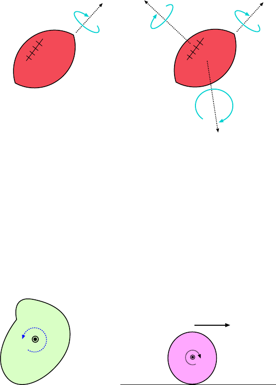
108 CHAPTER 8. ROTATIONAL KI NEMATICS
(a)
(b)
Figure 8.1: (a) Football thrown the right way. (b) Football throw n the way I always throw one. It has
several kinds of rotation all at once!
v
(a)
(b)
Figure 8.2: The kinds of (simple) rotations we will consider. (a) Object turns about a fixed axis. (b)
Rolling object turns about an axis which itself is in motion.
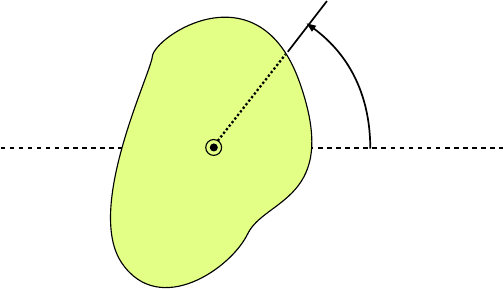
8.1. THE IMPORTANT STUFF 109
q
Figure 8.3: Orientation of a rotating object is given by the angle θ.
8.1 .2 Angular Displacement
The orientation of a rotating object is given by a single number, an angle θ, which can be
taken as the angle b etween some some radial marker on the object and some fixed axis, as
shown in Fig. 8.3.
Now, while we have so far measured angles in degrees (since they are easiest to visualize)
it turns out that it is now more convenient to measure angles in radians. Recall that there
are 2π radians in a full circle, i. e. 360 degrees:
2π radians = 360 degreees or π radians = 180 degrees (8.1)
Also keep in mind that 1 revolution just means that the object makes one full turn. To
convert between the different “units” for rotations, use
1 revolution = 360 degree s = 2π radians
The reason for using radians to measure angles is that it wil l be useful to talk about the
actual distance a point on a rotating objec t travels when the object rotates by an angle θ.
As shown in Fig. 8.4, a point at distance r from the axis travels a distance s when the object
rotates through an angle θ. There is a simple relation between t hese values: s = rθ, which
is true only when θ is measured in radians. Thus:
s = rθ With θ in radians! (8.2)
We will also refer to s as the “linear distance” through which the point travels, though of
course the actual path is the arc of a circle.
When an object rotates all points have the same angular displacement, but since the
points are at different r’s, the linear distances they travel are different.
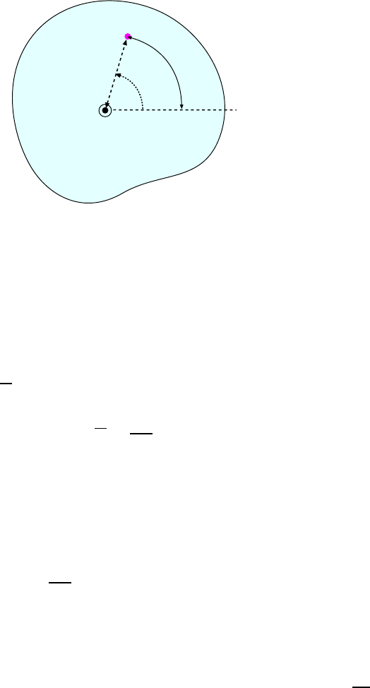
110 CHAPTER 8. ROTATIONAL KI NEMATICS
r
q
s
Figure 8.4: Object turns through an ang le θ; a point on the object at a distance r from the axis moves
through a distance s = rθ .
8.1 .3 Angular Velocity
We follow the same steps as in Chapter 2 to study the relation between angular displacement
and time.
If a rotating object turns through some angular displacement ∆θ in a time ∆t then the
average angular velocity ω for that period is
ω =
∆θ
∆t
(8.3)
(The symbol ω is the small Greek letter “omega”.)
As with our linear moti on, a much more interesting quantity is the instantaneous
angular velocity ω, which has the same kind of definition but applied to a very small time
interval ∆t and which than has meaning at a particular time t:
ω =
∆θ
∆t
For very small ∆t (8.4)
As used in these notes, angular velocity is a scalar (a single number) because of the
simplicity of our rotations; position is gi ven by a single angle θ. In advanced physics courses
where the rotations are more complicated it is necessary to treat angular velocity as a vector.
Since θ is measured in radians and t in seconds, the uni ts of ω ought to be
rad
s
and inde ed
if you are asked for an angular velocity you should give it with these units. But as we’l l see
if we stick by our practice of writing down all the units (including “rad”) we will run into
some inconsistencies later on, which basically come from the fact that our “radian” units is
mathematical in nature; there is no standard “radian” kept under glass in France anywhere.
Though opinions differ on this, my practice is that the symbol “rad” should taken as
optional, inserted just for clarity. When expressing an angular velocity or acceleration, one
8.1. THE IMPORTANT STUFF 111
should include it to emphasize that we are not using degrees. When we do a calculation
where the answer needs to come out in joules, then it should b e dropped. However it would
be OK (with me) to express an angular velocity in
1
s
= s
−1
.
When we set up our equations for angular displacement it will be simplest to say that at
time t = 0 the angular displacement is θ = 0.
8.1 .4 Angular Ac celeration
As we’ll see , when an outside i nflue nce acts on a rotating object the e ffect is that the
rotational motion (i.e. the angular velocity) changes and we now want a measure of how
rapidly the angular velocity changes with time. If the angular velocity of object has a change
∆ω in a time period ∆t We define an average angular acceleration α as:
α =
∆ω
∆t
(8.5)
But a more important quantity is the instantaneous angular acceleration, defined by
α =
∆ω
∆t
for very small ∆t (8.6)
The units of angular acceleration must be the units of angular velocity divi ded by those
of time, that is,
rad
s
s
=
rad
s
2
.
But as with angular velocity, I wouldn’t get upset i f you expressed it as
1
s
2
, treating the “rad”
as optional. Check with the l ocal Units Police officer.
8.1 .5 The Case of Constant Angular Accel eration
If α does not depend on time then for any time interval t (where we start counting time
from t = 0) we have
α =
∆ω
t
=
ω − ω
0
t
.
Here, ω
0
is the initial angular velocity of the object, that is, its angular velocity at t = 0.
This gives
ω = ω
0
+ αt (8.7)
We followed very similar steps in finding the equation v = v
0
+ at in one-dimensional motion
with constant linear acceleration. And in a similar way one can show that θ is given by
θ = ω
0
t +
1
2
αt
2
(8.8)
112 CHAPTER 8. ROTATIONAL KI NEMATICS
Here we measure θ such that θ = 0 at t = 0.
We can get other relations betwe en θ, ω and α with some algebra. One can show that
Eqs. 8.7 and 8.8 give:
ω
2
= ω
2
0
+ 2αθ (8.9)
And one can show
θ =
1
2
(ω
0
+ ω)t (8.10)
but you are cautioned that this equation holds only when we already know that α is constant.
8.1 .6 Relation Between A ngular and Linear Quantiti es
We’ve already mentioned that when the object turns by an angle θ a particular point on the
object at radius r travels a distance s, given by s = rθ.
Suppose an object is rotating with angular velocity ω. A point at radius r has speed v
which we can find from
v =
s
t
=
rθ
t
= r
θ
t
!
= rω
(Here we are really talking about a very small time interval t so that v and ω are the
instantaneous velocities.)
This gives us the relation between linear speed v and angular speed ω for the point:
v = rω (8.11)
We note that while all points of the object rotate at the same angular speed ω, because
they have different radii t hey will have different linear speeds v.
Finally we discuss t he acceleration of a point on the rotating object. This is little more
complicated, because there are two parts to the acceleration.
We have alr eady seen that when a particle undergoes uniform circular motion its acceler-
ation points toward the center of the circle and has magnitude a
c
=
v
2
r
. We can use Eq. 8.11
to express this as:
a
c
=
v
2
r
=
(rω)
2
r
= rω
2
(8.12)
But when the object has an angular acceleration there is also a component of the acce l-
eration in the tangential direction. This is because with an α which i s not zero, the linear
speed of the point is increasing as it travels on its circular path. Again taking a very small
time interval t, the tangential acceleration is given by
a
T
=
∆v
t
=
∆(rω)
t
= r
∆ω
t
= rα
That is,
a
T
= rα (8.13)
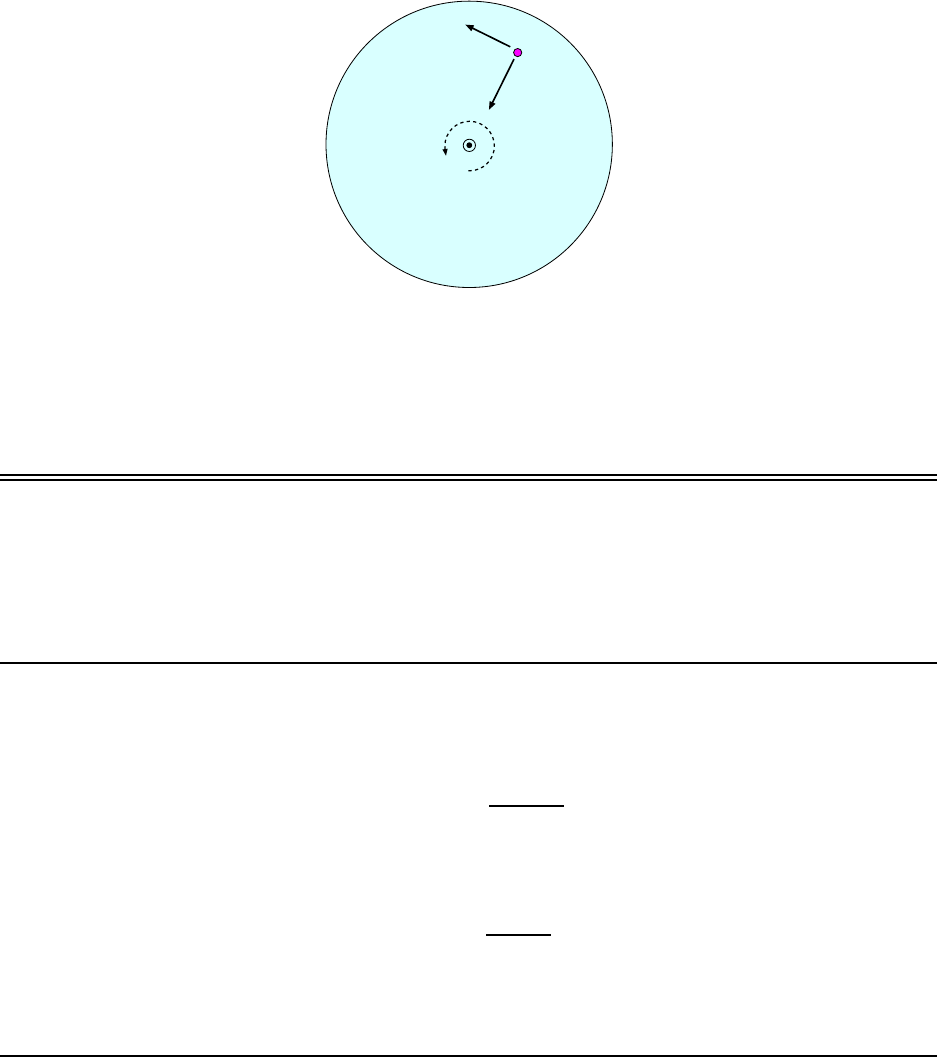
8.2. WORKED EXAMPLES 113
a
c
a
T
w, a
Figure 8.5: Acceleration of a point on a rotating object has centripetal and tangential components, a
c
and
a
T
.
So in general for a p oint on a rotating object, the acceleration has two components, as
illustrated in Fig. 8.5.
8.2 Worked Examples
8.2 .1 Angular Displacement
1. A rigid body turns through 1.85 radians. Expre ss this in degrees and revolutions
Use the fact that π radians equals 180
◦
, the n
1.85 rad = (1.85 rad)
180 deg
π rad
!
= 106 de g
Then, use the fact that 1 revolution = 2πrad to get
1.85 rad = (1.85 rad)
1 rev
2π rad
= 0.294 rev
8.2 .2 Angular Velocity and Acceleration
2. Long ago people listened to music which was stored on “phonograph records”.
These records turned at a rate of 33.3 revolutions per minute. Expre ss this
rotation rate in radians per second.
114 CHAPTER 8. ROTATIONAL KI NEMATICS
Use the relati ons 1 rev = 2π rad as well as 1 min = 60 s to convert the units:
33.3
rev
min
= (33.3
rev
min
)
2π rad
1 rev
!
1 min
60 s
= 3.49
rad
s
8.2 .3 Rotational M otion with Constant Angular Acceleration
3. A flywheel has a constant angular deceleration of 2.0
rad
s
2
. (a) Find the angle
through which the flywheel turns as it somes to rest from an angular speed of
220
rad
s
. (b) Find the time required for the flywheel to come to rest. [CJ7 8-19]
(a) The problem tells us that if we take the angular velociti es as positive, then we have
α = −2.0
rad
s
2
. Then if the init ial angular velocity is ω
0
= 220
rad
s
and it comes to re st (ω = 0)
as it turns through an angle θ, the relation between these quantities i s given by Eq. 8.9,
ω
2
= ω
2
0
+ 2αθ
so solving for θ,
θ =
(ω
2
− ω
2
0
)
2α
Plugging in the numbers,
θ =
(0)
2
− (220
rad
s
)
2
2(−2.0
rad
s
2
)
= 1.21 × 10
4
rad
(b) To find the time it takes the flywheel to come to rest, use Eq. 8.7,
ω = ω
0
+ αt =⇒ t =
(ω − ω
0
)
α
and we get
t =
(0 − 220
rad
s
)
(−2.0
rad
s
2
)
= 110 s
8.2 .4 Relation Between A ngular and Linear Quantiti es
4. A string trimmer is a tool for cutting grass and weeds. It utilizes a length of
nylon “string” that rotates about an axis perpendicular t o one end of the string.
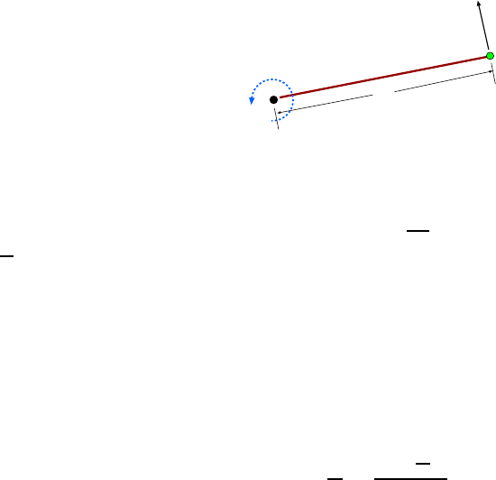
8.2. WORKED EXAMPLES 115
47 rev/s
54 m/s
r
Figure 8.6: Rotating string in Example 4.
The string rotates at an angular speed of 47
rev
s
, and its tip has a t angential speed
of 54
m
s
. What is the length of the rotating string? [CJ7 8-29]
The rotating string is shown in Fig. 8.6. The angular frequency of the string’s rotation
is
ω = 2πf = 2π(47 s
−1
) = 295 s
−1
We have the speed of the tip of the stri ng (which is a distance r from the axis), so fr om
Eq. 8.11 we can get the length of the string, r:
v = rω =⇒ r =
v
ω
=
(54
m
s
)
295 s
−1
)
= 0.183 m = 18.3 cm
The string is 18.3 cm long.
116 CHAPTER 8. ROTATIONAL KI NEMATICS

Chapter 9
Rotational Dynamics
9.1 The Important Stuff
9.1 .1 Introduction
Having worked with the kinematics of rotation in the last chapter we now move on to study
the dynamics of rotation. In effect, we have to r e-do that past chapters on dynamics (force,
energy and momentum) in the setting of rotating objects. We have our work cut out for us
and acc ordingly, this is a long chapter!
9.1 .2 Rotational Kinetic Energy
When an object turns around a fixed axis (as the y did in the last chapter) the individual
bits are in motion, so the object certainly has kinetic energy. Kinet ic ene rgy is always a
positive scal ar , so the kinetic energies of these little bits add up to give the kinetic ene rgy
of the whole object.
We would like to calculate the kinetic energy, but we must keep in m ind that even though
all parts of the object have the same angular velocity they have different speeds because they
lie at different distances from the axis. We will have to add up the kinetic energies of the
separate parts of the object; this is another derivation for which it is instructive (and easy)
to unde rstand all the steps.
Imagine the object is broken up i nto l ittle pieces, each indexed by the number i. Piece i
has mass m
i
, speed v
i
and sits at a distance r
i
from the axis, as shown in Fig.9.1.
The total kinetic energy of rotation is the sum of the kineti c energies of all the little bits:
KE
rot
=
X
i
1
2
m
i
v
2
i
117
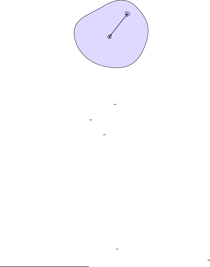
118 CHAPTER 9. ROTATIONAL DYNAMICS
r
i
m
i
Figure 9.1: A little piece of the rotating object ha s mass m
i
and is a distance r
i
from the axis.
Into this we substitute v
i
= r
i
ω, giving
KE
rot
=
X
i
1
2
m
i
(r
i
ω)
2
Now we take the common factors of
1
2
and ω
2
outside the sum and wri t e it as
KE
rot
=
1
2
X
i
m
i
r
2
i
!
ω
2
(9.1)
and now we focus on the quantity inside the parentheses in Eq. 9.1.
This quantity i s the sum over all the little pieces of the object of the mass of that piece
times its radius squared. (When the object is a continuous mass like a disc it is implied that
the pieces need to be very small!) This quantity i s called the moment of inertia of the
object
1
, and it is given the symbol I. Thus:
I =
X
i
m
i
r
2
i
(9.2)
As we will use it, the moment of inertia is a scalar. It units must be those of mass times
those of length squared, thus for physics they are
kg · m
2
There is no abbreviation for this.
Using this definition in Eq. 9.1 we have the simple expression
KE
rot
=
1
2
Iω
2
(9.3)
and we note that it looks like the expression for the kinetic energy of a particle, KE =
1
2
mv
2
.
1
Sometimes you will see it called the rotational inertia.

9.1. THE IMPORTANT STUFF 119
9.1 .3 More on the Moment of Inertia
Most of the time we are interested in the moment of iner t ia of some continuous object like
a rod or a disk, and for these shapes, even though we use the principle given in Eq. 9.2 we
actually need calculus to get the result.
So it is best just to give a short catalogue of formulae to use with the most comm on basic
shapes we’ll see in our problems.
Figures 9.2 and 9.3 give a set f or formulae for the moments of inertia for various shapes.
In all these cases we assume that the material of the object has uniform density. To use the
formulae, we need to know the mass of the object and one or two of its dimensions. Some
of the most commonly used formulae are:
I
hoop
= MR
2
I
disk
=
1
2
MR
2
I
solid sph
=
2
5
MR
2
(9.4)
It’s important to realize that the value of the moment of inertia depends on where we put
the axis. For example, for a uniform rod, the moment of inertia when the axis goes through
the middle is
1
12
ML
2
. But when the axis goes through the end of the rod, the moment of
inertia is
1
3
ML
2
.
There is a useful theorem which can give us the moment of inertia under a special
circumstance. Suppose:
• We know that moment of inertia of some object around an axis which goes through its
center of m ass, I
cm
.
• We want the moment of inertia around an axis which is parallel to that axis, a distance D
away from it.
Then we can get the desired moment of inertia from a sim ple formula,
I = I
cm
+ MD
2
, (9.5)
a formula which is calle d the Parallel Axis Theorem. The elements of the theorem are
illustrated in Fig. 9.4.
9.1 .4 Torque
When we arrived at Chapter 4 we asked the question: “Accelerations are what makes motion
interesting. . . what causes an object to accelerate?”. We do something analogous here: “An-
gular accelerations are the interesting feature of rotational motion; what makes a rotating
object accelerate?”
Actually, forces are still the cause for changes i n motion, but for our present purposes
the best answer is that changes in rotational motion are caused by a rotational version of
force called t orque. Torque has something to do with the force exerted on the object but it
also de pends on where the forces are exerted and their directions.
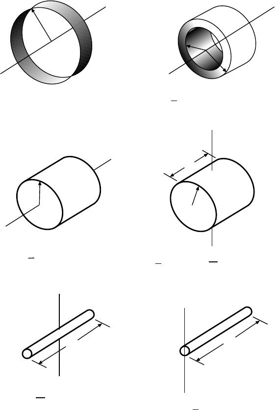
120 CHAPTER 9. ROTATIONAL DYNAMICS
R
R
1
R
2
R
R
L
L
L
(a)
(b)
(c)
(d)
(e)
(f)
MR
2
M(R
1
+R
2
)
1
2
2
2
ML
2
MR
2
1
4
ML
2
1
12
+
1
12
ML
2
1
3
MR
2
1
2
Figure 9.2: Some values of the moment of inertia for vario us shapes and choices of axes.
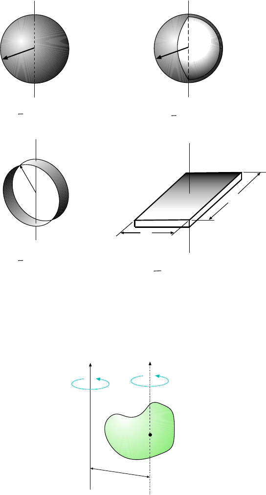
9.1. THE IMPORTANT STUFF 121
R
R
(a) (b)
R
(c)
(d)
a
b
MR
2
2
5
MR
2
2
3
MR
2
1
2
M
(
a
2
+b
2
)
1
12
Figure 9.3: Mo re moments of inertia.
cm
I
cm
I
D
M
Figure 9.4: The Parallel Axis Theorem: Axis through the cm gives I
cm
, and we want the moment of inertia
I about a new axis.
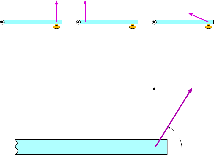
122 CHAPTER 9. ROTATIONAL DYNAMICS
F
F
F
(a)
(c)
(b)
Figure 9.5: Forces exerted on a door: (a) Force exerted far from the hinge, perpendicular to the door face.
(b) Force is exerted perpendicular to the door face but close to the hinge! (c) Force is exerted far from the
hinge but not perpendicular to the door face. Attempting to open a door using the forces in (b) or (c) will
only make you look fooli sh.
F
f
Fsin f
Figure 9.6: Only the perpendicular part of the force, F
⊥
contributes to the torque; F
⊥
= F sin φ.
Fig. 9.5(a) shows how one should e xert a force to open a door. Push on the end far away
from the hinge (axis) and push perpendicularly to the line which joins the axis to the point
of application. Exerting a force thi s way gives a large amount of torque on the door.
Figs. 9.5(b) and (c) show how not to open a door. I n (b) the force is exerted perpendicular
to the length of the door but it is too close to the hinge. In (c) the force is exerted far from
the hinge but not perpendicularly to the line joining hinge and the point of application.
When you go openi ng do ors, exert a force like the one shown in 9.5(a)!
The “thing” that makes the door rotate contai ns the magnitude of the force exerted (F )
and the distance from the axis (r), but is only the perpendicular part of the force (F
⊥
) that
matters, i.e. perpe ndicular to the li ne joining the axis and point of application, as shown in
Fig. 9.6.
The magnitude of the torque, τ is the product of F
⊥
and r:
τ = rF
⊥
= rF sin φ (9.6)
where φ is the angle be tween t he line from the axis the dire ction of the force.
We now work on the details of the definition of “torque”; it’s a little confusing.
Is it a vector or a scalar? In actuality it’s a vector, and if the force and line from the
axis lie in a certain plane, the dire ction of the torque is perpendicular to that plane, (which
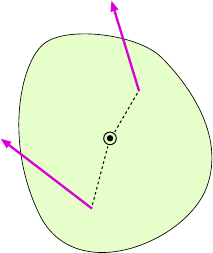
9.1. THE IMPORTANT STUFF 123
F
1
F
2
f
1
f
2
Figure 9.7: Given that our positive rotation direction is counter-clockwise, force F
1
gives a positive torque.
Force F
2
gives a negative torque.
we might call the z direction). For our present purposes, the rotations we consider are all
simple so we are only usi ng the z component of the torque. In that case we’re only talk ing
about a single number so we will treat torque as a number. But this number can be p ositive
or negative.
What about the units? From its definition the units must be those of force times those
of distance, i.e. N ·m. Now it is true that in Chapter 6 we said that this combination was a
“joule”. It wouldn’t be quite right to use that notation here because torque is a very di fferent
quantity from energy and the two quantities never really mix in any of our work. So it is
considered good practice to leave the units of torque as N · m.
Now we need to be more careful about the definition in Eq. 9.6. I t is really the magnitude
of the torque exerted on the object by the force F . Just as our angular displacements can
be positive or negative, torque wil l also bo positive or negative depending on whether the
force is making the object rotate in the positive or negative sense.
To avoid using more mathematics than we need, we’ll use the following convention: We
can use 9.6 to get t he magnitude of the torque; if the force would make t he object rotate in
the counter-clockwise direction, the torque is positive. If the force would make the object
rotate in the clockwise sense, the torque will be negative. Examples are shown in Fig. 9.7.
Of course, we can let “clock-wise” be the positive rotation direction, as long as we are
consistent.
With thi s in mind, we define the magnitude of torque as
|τ| = rF sin φ (9.7)
where φ is angle between the direction of the force and the line from the axis.
When we have several forces acting on a rotating object we will want to find the total
torque. Just add up the individual torques, making sure you get the signs right.
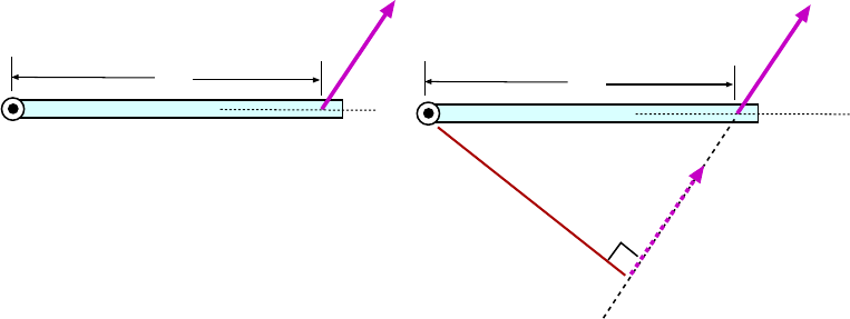
124 CHAPTER 9. ROTATIONAL DYNAMICS
l
f
f
F
F
f
F
(a)
(b)
r
r
Figure 9.8: (a) Force F pulls at angle φ from the radial line. (b) We drop a “line of action” along the
direction of the force and make a perp endicular “lever arm” from the axis. Now the (same) force pulls
perpendicularly to the lever arm. Lever arm has length ` = r sin φ.
9.1 .5 Another Way to Look at To rque
Another way to arrive at our definition of torque, Eq. 9.7, advocated in some textbooks is
as follows.
Again start with a rotating system like a door with a force of magnitude F pulling at a
distance r and angle φ, as in Fig. 9.8(a). We know that things are simple when the force
is pulling perpendicularly to the line from t he axis, and we can do some t hing interesting to
create t his condition.
Fig. 9.8(b) show how to do t his. Draw a line along the direction of the force such we can
drop a new line from the axis which is perpendicular to the force. Now we have the simple
situation f or torque . The length of this new line is ` and is called the l ever arm for the
force in question. We then want to have τ = `F for our formula. But is that the same as
what we had before?
Fig. 9.8(b) shows that it is. Since ` = r sin φ we get
τ = `F = (r sin φ)F = rF sin φ
and it’s t he same as before.
9.1 .6 Newton’s 2nd Law for Rotations
What is torque good for? If the torque on a object is greater then the angular acceleration
that the object wil l undergo is greater; that much is obvious, but what is the relation between
the two?
We can get a hint from considering the motion of single mass point m around an axis
at a distance r. Suppose a single force F acts on this mass in the tangential direction.
9.1. THE IMPORTANT STUFF 125
Then Newton’s 2nd law gives F = ma, a being the acceleration in the tangential direc t ion.
Multiply both sides by r and get rF = mar.
Now make some substitutions in this last equation. Since the force is applied at 90
◦
to
the radial line, it gives a torque τ = rF . Also the linear accel eration a is tnagential and is
related to its angular acceleration by a = a
T
= rα. This gives us:
τ = m(rα)r =⇒ τ (mr
2
)α
Now the moment of inertia for a single point mass m at a distance r is I = mr
2
. Making
this substitution in t he last equation gives
τ = Iα
While this li t tle derivation doesn’t show very much it turns out that one can show that
the result is general: When we have a bunch of (external) forces acting on a rotating object
giving some net torque τ
net
, the net torque is related to the moment of inertia and angular
acceleration by
τ
net
= Iα (9.8)
This relation is often called N ewton’s 2nd l aw for rotations and inde ed it strongly
resembles the original version of Newton’s 2nd law: Compare F = ma with τ = Iα. In the
second one, torque plays the role of force and the moment of inertia plays the role of the
mass. Of course, α corresponds to a as we saw in the last chapter.
9.1 .7 Solving Problems with Forces, Torques and Ro tating Ob-
jects
Knowing how rotating objects behave we can now solve problems which involve (idealized)
rotating systems. Ofte n the problem will include a pulley or wheel over which a string passes.
The pulley will have mass, and that will be an i mportant aspect of the problem but generally
we will ignore any fricti on in the bearings of the pulley. (When we consider it, it wil l give a
torque which opposes its rotational motion.)
We will now have to make free–body diagram (i.e. draw the damn picture) for the
rotating objects as well. For the rotating elements the diagram will show the forces acting
and where they are applied .
Two typical elements in these problems are shown in Fig. 9.9. In (a) a string is wrapped
around a pulley or radius R. Ther e is a tension T in the string; the string rol ls off the pulley
tangentially. We can treat this system as if a force of magnitude T is pulli ng at the edge
of pulley, at right angles to the radial line . Then the torque on the pulley (from the string
force) is T R sin 90
◦
= T R.
We will use the fact that the linear motion of the edge of the pulley (where the string
rolls off) is the same as that of the string itself.
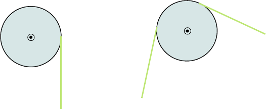
126 CHAPTER 9. ROTATIONAL DYNAMICS
T
T
2
T
1
(a)
(b)
Figure 9.9: (a) String wrapped around a pulley; tension T gives a torque on the pulley. (b) String is in
contact with pulley; tensions on the different sides are not the same.
Another one is shown in (b). Here a string passes over an ideal pulley and does not slip,
so again the linear moti on of the edge of the pulley is the same as that of the string. Now,
in the case that the pulley has mass, the parts of the string on either side of the pulley have
different tensions. the string forces can b e treated as forces applied at the edge, t angent to
the pulley, so that in (b) the (clock-wise) torque from the string is
τ = T
1
R − T
2
R = (T
1
− T
2
)R
9.1 .8 An Example
The following example will give show how we can solve problems involving rotating objects.
A string is wrapped around a pulley of mass M and radius R. The string is attached
to a mass m; the mass is released. Find the acceleration of the mass as it falls. Treat the
pulley as if it were a uni form disk of radius R.
The basic situation is shown in Fig. 9.10. The mass will fall with an acceleration that
we expect will be somewhat less than g. As it falls the pulley will turn and since the motion
of the e dge of the pulley is the same as that of the string, the edge of the pulley will have a
tangential acceleration and the pulley will have an angular acceleration; it will rotate faster
and faster.
We have to analyze the force with diagrams; we wi ll now have a diagram for the block
and one for the pulley. First, the block. Forces on the blo ck are shown in Fig. 9.11(a).
Gravity mg points down and the string tension T pulls upward. Since the motion of the
mass is downward, we’ll let “down” be the p ositive direction for simplicity and let a be the
downward acceleration of the mass. Then Newton’s 2nd law gives:
mg − T = ma (9.9)
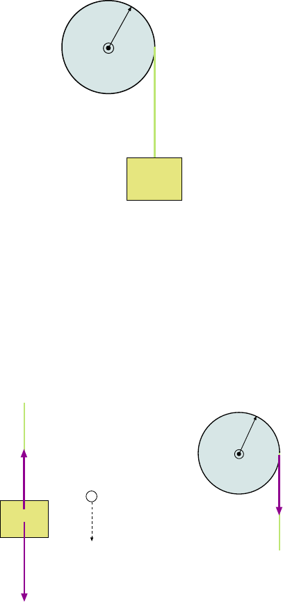
9.1. THE IMPORTANT STUFF 127
m
R
M
Figure 9.10: Mass hangs from a string which is wrapped around a wheel.
T
(a)
(b)
T
mg
R
+
Figure 9.11: (a) Forces on the bl ock. Positive direction of motion will be taken as downward for simplicity.
(b) Fo rce on the wheel.
128 CHAPTER 9. ROTATIONAL DYNAMICS
Now look at the forces acting on the pulley, shown in Fig. 9.11(b). The string tension
acts to give a tangential force T at the edge of the wheel, and hence a torque of RT . That’s
the only force which gives a torque around the wheel’s axis. Note, for this picture, we are
taking “clock-wise” as the positive rotation dir ection. (I know, that isn’t our convention.
So sue me.) This choice makes things consistent with the choice (downward) for the block’s
motion. Anyways, Newton’s 2nd law for rotation gi ves
τ = RT = Iα (9.10)
We can treat the pulley as a uniform disk of radius R, so we can substitute I =
1
2
MR
2
here. Also, we recall that the tangential acceleration of the edge of the wheel is the same as
that of the string and of the mass m, namely a. Then we can write:
a = a
T
= Rα =⇒ α =
a
R
Now make these two substitutions in Eq . 9.10. Then we have:
RT =
1
2
MR
2
a
R
=
1
2
MRa =⇒ T =
1
2
Ma (9.11)
Use this to substitute for T in Eq. 9.9 and get
mg −
1
2
Ma = ma (9.12)
Now do some algebra to solve for a:
mg =
1
2
M + m
a =⇒ a =
mg
1
2
M + m
(9.13)
This result makes sense if we set M = 0. We find that the formula then gives a = g. This
is what we should get because that is the case where the hanging mass is really attached to
nothing and falls f r eely under gravity.
9.1 .9 Statics
From Chapter 7 and t he current chapter we have some rules about the total forces and
torques on objects which, for our present purposes can b e expre ssed as:
If the center of mass of an object is at rest, then the total external force on
the object must be zero.
If an object is not rotating then the total torque on it must be zero.
Actually the second of these statements is true for any choice of an axis which as we’ll
see can be used to make problem–solving a little easier.
9.1. THE IMPORTANT STUFF 129
Now, there many situations in the world when we we’d like some object to be absolutely
motionless. For example, since gravity acts on all objects on the earth we m ight need to hold
them up and make sure the y don’t fall; we need to do t his with various forces of support
and we need to know what forces are require d to support the objects.
Problems of this sort can be very complicated if the structures and the applied forces
are messy; there is a whole area of engineering devoted to this, known as “Statics”. We will
work with some very simpl e e xamples of this sort of problem.
The strategy for solving such problems is to first draw the force diagram for the object.
(You can’t do these problems without a diagram.) Include the dime nsions of the objects
and where the forces are applied, and if possible the directions of the f orces. Then apply the
conditions:
X
F
x
= 0
X
F
y
= 0
X
τ = 0 (9.14)
(We’ll only work in two dimensions so the force condition just has two components.) As
mentioned, for the condition on the torques you can choose any point on the object to server
as an axis.
To make the math easier it is often useful to put the axi s at a place where one or more
unknown forces are applied; since those forces will give no torque about that axis they will
not appear in the torque equation.
9.1 .10 Rolling Motion
A very common kind of motion is when a round object like a cylinder or a sphere rol ls
without slipping on a surface. This means that as the object moves the arc length around
its edge matches one-to-one with the distance travelled linearly, as indicated in F ig. —.
Because of this match-up, we can relate the quantities f or linear motion with the angular
quantities. First, if the object turns through an angle θ while rolling the linear distance
travelled by the center of the object is
x
c
= Rθ (9.15)
where R is the radius of the object. The velocity of the center and angular velocity of the
object are related by
v
c
= Rω (9.16)
And finall y the linear acceleration of the center and angular acceleration of the object are
related by
a
c
= Rα (9.17)
These are the values of the li near speed, velocity and acceleration of the center of the
object. The instantaneous velocities of the other parts of the object are different: The point
130 CHAPTER 9. ROTATIONAL DYNAMICS
in contact wi th the surface has an instantaneous veloc ity of zero which the top point has a
speed of 2v
c
in the forward direction.
Because the rolli ng object is in contact with the surface there m ay be a f orce of friction
from the surface. If so, it is a force of static friction because the very bottom of the rolling
object has no velocity relative to the surface . (And recall that the normal force of the surface
only gives us the maximum value of the static f r iction force.)
A rolling obj ect has kinetic e nergy, of course. One can show that if an object with
moment of mass M and moment of inerti a I is rolling so that the speed of its center is v
c
and its angular velocity is ω, its kinetic energy is
KE =
1
2
Mv
2
c
+
1
2
Iω
2
= KE
trans
+ KE
rot
(9.18)
that is, it is the sum of two parts: One part comes from the translational motion of the
center, and the other comes from the rotational motion of the object about its center.
Sometimes in solving a problem, the total KE in Eq. 9. 18 for a rolling object can be
expressed more simply if we know the expression for the moment of inertia. For example,
suppose the object is a uniform cylinder. In that case, I =
1
2
MR
2
and since ω = v
c
/R we
get
KE
total
=
1
2
Mv
2
c
+
1
2
Iω
2
=
1
2
Mv
2
c
+
1
2
(
1
2
MR
2
)
v
c
R
2
=
1
2
Mv
2
c
+
1
4
Mv
2
c
=
3
4
Mv
2
c
9.1 .11 Example: Round Object Rolls Down Slope Without Slip-
ping
An important example of rolling motion is that of a round symmetrical object rolling down
a slope inclined at angle |thet a, as illustrated in Fig. 9.12 (if for no other reason than that
it is easy to set up in the lab). The object has mass M, radius R and moment of inertia I
about its center.
We would like to find the acceleration of the center of the object. Recall that when we
did this problem for a mass sliding down the slope without frict ion we got a = g sin θ; but
this is a di fferent problem.
The forces acting on the object are shown in Fig. 9.13. Gravity acts with magnitude Mg
downward and we can treat its force as acting at the center of the object. (Thinking ahead,
we split the vector into parts “down the slope” and perpendicular to the slope as shown in
Fig. 9.13. Then we work with these comp onents in Newton’s laws. ) The normal force of
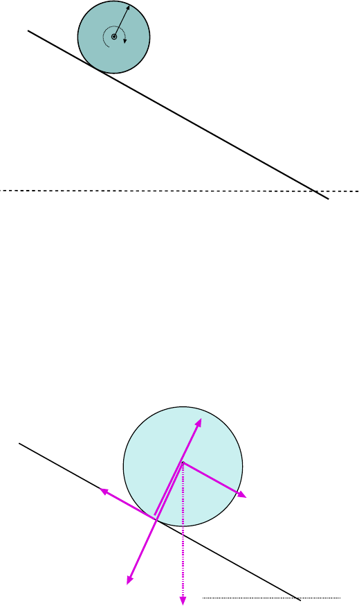
9.1. THE IMPORTANT STUFF 131
q
M
R
I
Figure 9.12: Example: Object with mass M radius R and moment of inertia I rolls (without slipping)
down a slope inclined at θ above the horizontal.
q
Mg
Mg sinq
Mg cosq
f
s
F
N
Figure 9.13: Forces a cting on the round object as it rolls down the slope. The downward force of gravity
Mg has been split up into its components along/perp to the slope.
132 CHAPTER 9. ROTATIONAL DYNAMICS
the surface F
N
is applied at the point of contact, as is the force of friction f
s
which acts
along the surface in the direction shown. (Actually, it may not be cl ear that fri ction acts in
the backward direction, but that will be c lear later.)
We will consider the forces acting on t he object and apply the re gular version of Newton’s
2nd law. Then we will consider the torques acting about the center of the wheel and apply
the rotational version of Newton’s 2nd law. Eventually we will get a
c
.
Take “down the slope” as the positive direction. The forces acting down the slope are
the component Mg sin θ from gravity minus the force of friction f
s
which acts up the slop e.
Newton’s 2nd law gi ves:
Mg sin θ − f
s
= Ma
c
(9.19)
Next the torque: This time we will take “clock-wise” to be the positive rotation directi on
(to be consistent with the linear acceleration) and sum of the clock-wise torques will equal
Iα. Sinc e gravity acts at the center and the normal force acts along a line through the center
(so φ = 0), only the friction force gives a torque about the center. It act perpendicularly to
the radial line, at a distance R, so:
τ
net
= f
s
R = Iα (9.20)
Lastly, by Eq. 9.17, a
c
and α are related:
a
c
= Rα (9.21)
Equations 9.19, 9.20, and 9.21, have three unknowns (f
s
, α and a
c
) so we can solve for
them. Putting 9.21 into 9.20 gives
f
s
=
Iα
R
=
I(a
c
/R)
R
=
Ia
c
R
2
and putting this into 9.19 gives
Mg sin θ −
I
R
2
a
c
= Ma
c
Doing some algebra to get a
c
, we get:
Mg sin θ =
M +
I
R
2
a
c
and finally (drum roll), the answer:
a
c
=
Mg sin θ
M +
I
R
2
(9.22)
9.1. THE IMPORTANT STUFF 133
We can make it a little cleaner by dividing top and bottom by M, and t hen we have:
a
c
=
g sin θ
1 +
I
M R
2
(9.23)
and then we see that since the denominator is bigger than 1 the acceleration of the object
must be smaller that g sin θ, the “sliding” value. Also if we could fix the value of M but
make the moment of inertia larger, a
c
would get smaller.
Some specific examples might be useful here. If the rolling object is a uniform cylinde r
then I/(MR
2
) =
1
2
and we get:
a
c
=
g sin θ
1 +
1
2
=
g sin θ
3
2
=
2
3
g sin θ
or if the object is a sphere then I/(MR
2
) =
2
5
and the n
a
c
=
g sin θ
1 +
2
5
=
g sin θ
7
5
=
5
7
g sin θ
Note that in both of these results the actual mass and radius do not appe ar although the
results depend on the shapes of the objects; a ny uniform cylinder wil l roll down the slope
with acceleration
2
3
g sin θ. Since
5
7
>
2
3
a uniform sphere has a larger acceleration than the
cylinder in rolling down the slope.
9.1 .12 Angular Momentum
And we conclude with the rotational version of mome ntum.
We have found that the m ass m from linear dynamics corresponds to the m oment of
inertia I in rotational dynamic s, and the velocity v corresponds to the angular velocity ω.
We found in Chapter 7 that a useful quantity in linear motion was the momentum, p
x
= mv
x
.
If we had to come up with the rotational version of this quantity (for whatever reason) it
would have to be Iω, and that is what we will use for the rotational version of “momentum”
. For our simple rotating systems, we define the angular momentum L as:
L = Iω (9.24)
Angular momentum (as we will use it, for our simple rotations) is just a si ngle number,
although as with angular velocity and torque we’re really talking about the z component of
a vector. Its units are those of I tim es those of ω (without the “rad” marker, i.e.
1
s
), thus
they are:
kg · m
2
·
1
s
=
kg·m
2
s
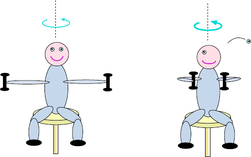
134 CHAPTER 9. ROTATIONAL DYNAMICS
(a)
(b)
Figure 9.14: (a) Minimalist man holds weights in outstretched arms. Initially, he has a small rate of
rotation. (b) Man pulls weights inward; mom ent of inertia of system is smaller and rate of rotation is larger.
Again, there is no common abbreviation for this unit.
We will refer t o our previous quantity p = mv as linear momentum to keep things
straight.
Recall that the reason that linear momentum was so useful was that it was conserved
for an isolated system. That is, if the net external force acti ng on a system of particles was
zero, their total linear momentum stayed the same.
A similar thing is true for the rotational case; the terms just translate over from linear
to r otational language:
If there is no net external torque on a system of objects, their total angular
momentum stays t he same.
This principle is known as the c onservation of angular m omentum.
A familiar example of the application of this principle is that of a spinning ice skater who
is initially turning at a slow rate with her arms outstretched and then turns much faster
when she pulls them in. One can also show the effect by resting on a turntable or rotating
stool and holding two weights in your outstretched arms, as shown in Fig. 9.14. If you are
given a small rotation rate at first you can make yourself spin much faster by pulling in your
arms, so much so that it is often hard to stay on the turntable!
What is going on here?
Both before and after the arms are pulled in, the angular momentum of the turning
system is given by L = Iω. Since there are no (significant) external torques on the system,
the product of L and ω will remain the same. But when the arms are pulled in the moment
of inertia I decreases so then ω — the rate of turning — must incre ase.

9.2. WORKED EXAMPLES 135
Using some math, if I
i
and I
f
are the initial and final moments of inertia and ω
i
and ω
f
are the initial and final angular velocities, then conservation of angular momentum gives
I
i
ω
i
= I
f
ω
f
so that the final angular velocity is
ω
f
=
I
i
I
f
!
ω
i
that is, the final angular velocity is bigger than the initial angular velocity by a factor given
by the ratio of the moments of iner tia.
A word of caution about this example: It is true that angular momentum is conserved
as I changes, but in general the kinetic energy is not conserved. The rotating man has
more kinetic e nergy after pulling his arms inward. You c an appreciate this if you do the
demonstration yourself; you will fee l yourself doing work as you pull your arms inward.
increasing the energy of the rotating system.
9.2 Worked Examples
9.2 .1 The M oment of Inertia and Rotational Kinetic Energy
1. A horizontal 150–kg merry-go-round of radius 2.0 m is turning at a r ate of
32.0 rpm. What is its kinetic energy? (Assume the merry-go-r ound is a uniform
disk. )
Find t he angular velocity of the merry-go-round: Converting from revolutions per minute
to r adians per second,
(32.0
rev
min
)
1 min
60 sec
2π rad
1 rev
!
= 3.35
rad
s
Using the formula for the moment of inertia of a uniform disk from Eq. 9.4, we have:
I =
1
2
MR
2
=
1
2
(150 kg)(2.0 m)
2
= 300 kg · m
2
and from Eq. 9.3, the kinetic energy is
KE =
1
2
Iω
2
=
1
2
(300 kg · m
2
)(3.35
rad
s
)
2
= 1.68 × 10
3
J
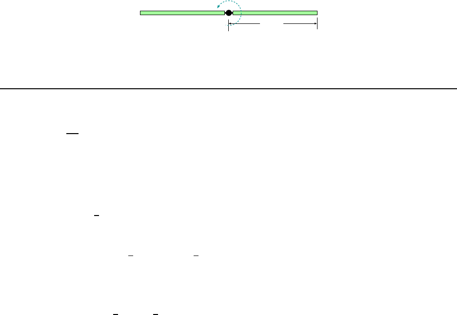
136 CHAPTER 9. ROTATIONAL DYNAMICS
6.7 m
240 kg
w = 44 rad/s
Figure 9.15: Helicopter blades for Exa mple 2.
2. A heli copter has two blades each of which has a mass of 240 kg and can be
approximated as a thin rod of length 6.7 m. The blades are rotati ng at an angular
speed of 44
rad
s
. (a) What is the total moment of inertia of the two blades about
the ax is of rotation? (b) Determine the r otational kinetic energy of the spinning
blades. [CJ7 9-4 6]
(a) We sketch the system i n Fig. 9.15. From our formulae for the moment of inertia of basic
shapes, we re call that the moment of ine r tia of a thin stick rotating about an axis at one
end of the stick is
1
3
ML
2
where L is the length of the stick. We have two such sticks in our
simple treatment of the helicopter blades, so the total moment of inert ia i s
I
blades
= 2
1
3
ML
2
= 2
1
3
(240 kg)(6.7 m)
2
= 7.18 × 10
3
kg · m
2
(b) A nd now to get the kinetic energy of the rotating blades, use Eq. 9.3:
KE =
1
2
Iω
2
=
1
2
(7.18 ×10
3
kg · m
2
)(44 s
−1
)
2
= 6.95 × 10
−6
J

Chapter 10
Oscillatory Motion
10.1 The Important Stuff
10. 1.1 Introduction
All right, back to one-dimensional motion. (Eh? Haven’t we done e verything that can b e
done with one-dimensional motion?)
In Chapter 6 we encountered the “spring force”, a force which is proportional to the
displacem ent and opposes it. As you will surely recall, the force from an “ideal” spring
followed the f ormula given in Eq. 6.8,
F = −kx (10.1)
where k was called the “force constant” of the spring and x is the displacement of the end
of the spring from the equilibrium position. You’ll also recall that the energy stored in the
spring is PE =
1
2
kx
2
.
In Chapter 6 we had masses bump into springs and exchange energy with them. Now
we’ll do something a l ittle different. We’ll attach a mass to the end of a spring, pull the mass
back a little ways (a distance A) and then release it, as shown in Fig. 10.1. (The surface on
which the mass is sl iding is frictionless!)
What do we expect the ensuing m otion to be like?
Since the mass gets pulled inward when the spring is stretched and gets pushed outward
when the spring is compressed we expect the motion to be re presented by something like the
x vs. t graph in Fig. 10.2.
10. 1.2 Harmonic Mo tion
The graph in Fig. 10.2 shows how the mass would move if the spring i s ideal and obeys the
force law F
spr
= −kx. The curve is “sinusoidal” meaning that it fol lows the basic form of
137
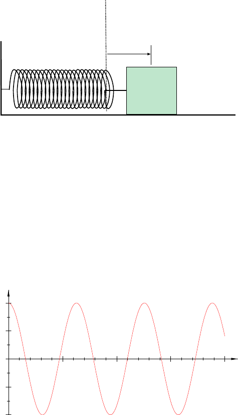
138 CHAPTER 10. OSCILLATORY MOTION
A
m
k
Figure 10.1: Mass m attached to spring of force constant k is pulled back a distance A and released.
-1.00
-0.50
0.00
0.50
1.00
x
0.0 5.0 10.0 15.0 20.0 t
Figure 10.2: Motion of mass on the end of a spring.
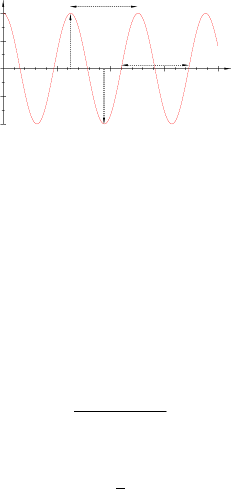
10.1. THE IMPORTANT STUFF 139
T
T
A
A
t
x
A
-A
Figure 10.3: Period T and ampli tude A of the motion of the mass on a spring.
the sine or cosine func t ions (I hope) you’ve seen in m ath.
When the motion of an object depends on time in this sinusoidal fashion, we say that
the obje ct is undergoing harmonic motion and that the physical system produc ing such a
motion is a harmonic oscillator.
The maximum distance which the mass goes outward f rom the eq uilibrium point is the
same as the maximum distance it goes inward. This distance is called the amplitude of the
motion. In Fig. 10.3 the amplitude is indicated by A. (For the mass’s motion the amplitude
is a length and is measured in meters.)
Then there is the amount of time required for the mass t o make one full oscillation, that
is, to go back and forth and return to a place where its motion wil l repeat itself. This is the
period of the motion, and it is indic ated (twice ) on Fig. 10.3. The p eriod T is a time and
is measured in seconds.
A related number describing the rapidity of the oscillations is the number of oscillations
the mass will make in a given time period; thi s is called the frequency of the oscillations:
f =
(# of oscillations)
time
(10.2)
The frequency is the inverse of time divide d by oscillations; but the time for each oscil-
lation is t he perio d T , so that f is the inverse of T :
f =
1
T
One must be careful with the units of f. Even though it is the inverse of a time one should
always express f in te r ms of oscillations (or cycles) per second. It is true that “oscillations”
is not really a fundamental unit but it is important to distinguish frequency from angular
velocity ω because we will find that the two quantitie s are related.
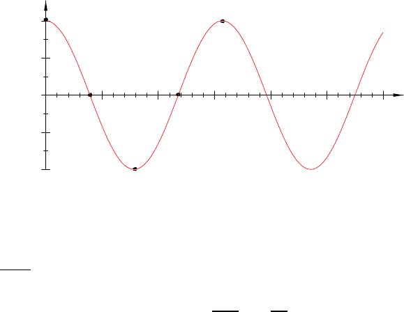
140 CHAPTER 10. OSCILLATORY MOTION
a
b
c
d
e
t
x
Figure 10.4: Points
In pl ace of
cycles
s
we c an also use shorter notation “Hertz”; thus:
1 Hz = 1
cycle
s
= 1
osc
s
10. 1.3 Displaceme nt, Velocity and Acceleration
We now look at the graph of x vs. t in greater to understand what i s happening with the
position, velocity and acceleration of the mass.
In Fig. 10.4 the plot of the motion is given over a couple cycles wit h some imp ortant
points marked (a)–(e).
At point (a) the mass is “released”, meaning that its initial velocity is zero. At this point
the displacement is a maximum. The acceleration of the mass is negative and takes on its
maximum size (magnitude) at this point because the spring force has maximum size at this
point.
At point (b) the displacement is z ero; here the mass is zipping through the equilibrium
position, where the spring has its natural length and ex erts no force. the velocity is negative
and has its m aximum size at this point. The acceleration is zero here.
At point (c) the mass has gone as far inward as it’s going to go; the displacement here is
negative and has the maximum size. The velocity is zero at this point. The acceleration i s
positive and has its maximum value.
At point (d) the mass is once again at the equil ibrium point so that the displacement x
is zero. But the velocity is now postivie and has the same maximum size as it did before at
this point. Since the spring is undistorted here the force and acceleration are zero.
At point (e) the motion is the same as it was at (a), i.e. maximum displacement, zero
velocity, maximal (negative) acceleration.
From here on the motion repeats.
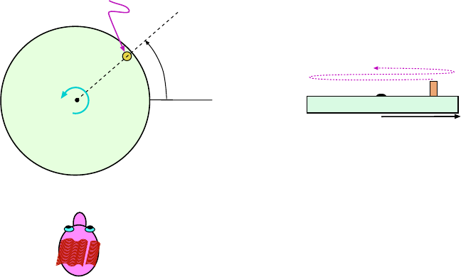
10.1. THE IMPORTANT STUFF 141
q
peg
A
(a)
(b)
Figure 10.5: Reference circle. (a) Top view of you with your bad haircut looking at the turning wheel
along its edge. Wheel has a peg located at its edge, at r = A. (b) What you see when you look at the wheel;
peg seems to move back and forth along a line.
10. 1.4 The Reference Circle
We can get some useful insight into the motion of the oscil lating mass by relating it to the
motion of a mass in uniform circular motion.
Imagine that we have a wheel of radius A whi ch turns at a constant rate; at the edge of
the wheel is a peg. Then imagine that you are looking at the turning wheel from the side,
i.e. le vel with the surface of the wheel. This is shown in Fig. 10.5(a). What you would
see in shown in Fig. 10.5(b); you would see the profile of the peg moving back and forth
horizontally, oscillating much like the mass on the of the spring. . . except that here there’s
no spri ng!
It turns out that the motion of the peg is exactly like that of the mass on the spring; in
both cases the object moves between x = −A and x = +A with a sinusoidal depende nce on
time. For the case of the p eg we can see this with a little m ath. Suppose the reference wheel
turns at a constant angular velocity ω then (as usual) assuming θ = 0 at t = 0, then θ is
given by θ = ωt.
Now the x coordinate of the peg ( which is all the man in Fig. 10.5(a) can see) is given
by x = A cos θ (see Fig. 10.6.) Putting these relations together, we have
x = A cos(ωt )
and for this relation the graph of x vs. t is a sinusoidal curve.
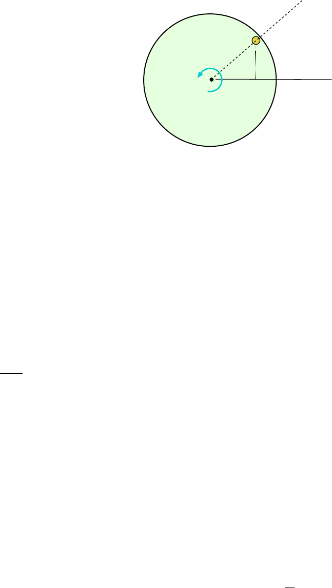
142 CHAPTER 10. OSCILLATORY MOTION
q
w
A
x
x = Acosq
q = wt
Figure 10.6:
Thinking of the reference circle we can associate an angular velocity ω wi th the motion
of an oscillator. This makes sense even though the mass in question really moves back and
forth along a line, not in a circle.
The angular velocity ω we associate with the oscillator and its frequency are related.
Every time the mass on the spring makes one full cycle the corresponding peg on the whee l
turns through 2π radians. This means that the angular velocity ω (in radians per second)
must be 2π tim es as large as the frequency f (in cycles per second) so that:
ω = 2πf ( 10.3)
But here I will repeat the c aution about the units given before: Eq. 10.3 seems to say that
both ω and f have the same units, but to avoid confusion we should always ex press f in
cycles
s
or Hz.
When we speak about an oscil lator we say t hat ω is the angular frequency of t he
oscill ator, as distinguished from the plain old frequency f.
We can use the reference circle to derive some useful formulae about oscillatory motion
from the fact that the man watching the peg on the wheel sees only the sideways (x) part of
the peg’s motion, and thus only the x components of its velocity and acceleration vectors.
When the peg is at the θ = 90
◦
position, as shown in Fig. 10.7(a), the velocity vector (which
always has the same magnitude, namely v = ωA)) is pointing sideways so that the man sees
the mass with a speed of |v
x
| = v
max
= ωA. So the largest speed of the mass is related to
the amplitude and frequency by
v
max
= ωA = 2πfA (10.4)
Next , consider the “view” of the mass when it i s at the θ = 0
◦
position, as in Fig. 10.7(b).
The man “sees” zero velocity but he sees the maximum size of the acceleration. The accel-
eration vector of the peg always has magnitude a
c
=
v
2
A
and here the m an sees a sideway s
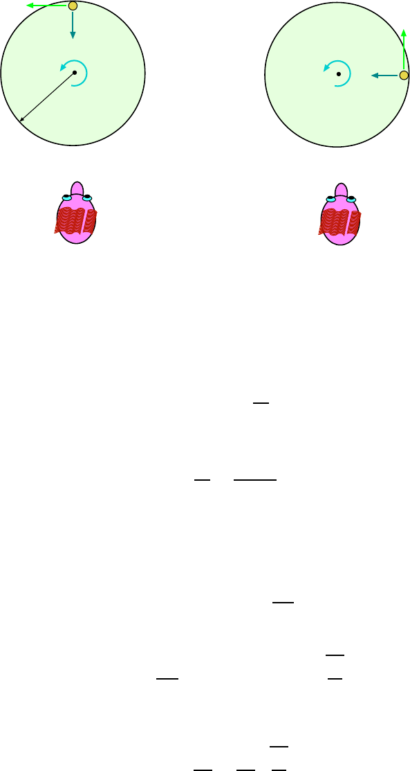
10.1. THE IMPORTANT STUFF 143
(a)
w
v
a
(b)
w
v
a
A
Figure 10.7: Man with big nose and bad haircut can only “see” the sideways components of the velocity
and acceleration vectors. (a) When the peg is at the θ = 90
◦
position m an sees the peg with maximum
velocity and zero acceleration. (b) When p eg is at the θ = 0
◦
position man sees the peg with zero velocity
and maximal acceleration.
acceleration a
x
of this size. So the maximum acce leration is
|a
x, max
| =
v
2
A
But now using v = ωA we get
|a
x, max
| =
v
2
A
=
(ωA)
2
A
= ω
2
A (10.5)
But the sideways motion of the peg is the same as that of the corresponding mass on a
spring, and when the mass is at the “far” position (the 0
◦
position for the peg) the f orce of
the spring has magnitude kA. Then from Ne wton’s 2nd law t he acceleration at the “far”
position the value
|a
x
| = |F
x
|/m =
kA
m
which is the same as the a
max
in the equation before it. Equating the two we find
ω
2
A =
kA
m
=⇒ ω =
s
k
m
(10.6)
and so a mass m osci llating on a spring of f orce constant k the frequency of the motion is
given by
f =
ω
2π
=
1
2π
s
k
m
(10.7)
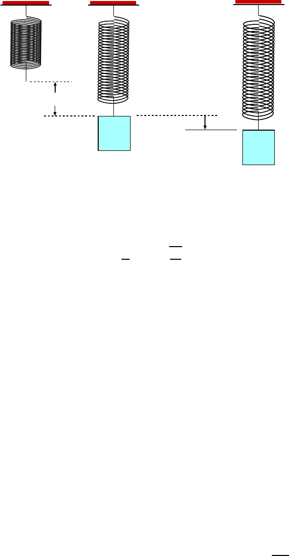
144 CHAPTER 10. OSCILLATORY MOTION
k
m
x
m
(a)
(b)
k
Figure 10.8: (a) Mass is attached to the end of a vertical spring; the spring stretches from its original
length so as to support the mass. (b) Mass will now oscillate around the new equilibrium position.
and the period of the motion is
T =
1
f
= 2π
r
m
k
(10.8)
The answer is a little surprising because the amplitude of the motion (A) does not appear
in it. So if we start the oscillations by pulling t he mass back by any distance A the frequency
of the oscillations is the same! (Recall the assumption about the spring behaving ideally; if
the spring doesn’t follow F
x
= −kx then we can’t make this statement.)
It might seem as though with a larger amplitude the period would be greater (the mass
has to move farther), but that’s not the case!
10. 1.5 A Real Mass/Spring System
Since the mass on the spri ng in Fig. 10.1 needs to slide on a f r ictionless surface, the setup
illustrated would be difficult to set up in the lab even if we could get a spring which has
ideal behavior. With f r iction present the system would lose mechanical energy and come to
a halt.
It turns out that one can get (basically) t he same behavior by suspending the mass from
a spring and letting the mass bob up and down as shown in Fig. 10.8. When the mass hangs
from the spring with no motion, as in Fig. 10.8(a), the spring is stretched so as to give a force
to hold the mass up, i.e. the spring force equals the weight of the spring. The elongation x
is given by
|F
spr
| = F
grav
=⇒ kx = mg =⇒ x =
mg
k
Now if mass is given a little tap it will oscillate up and down around this new position
10.1. THE IMPORTANT STUFF 145
(as shown in F ig. 10.8(b)) with the same freq uency as in the horizontal case, that is, T =
2π
q
m/k. It might seem surprising that the frequency doesn’t depend on the value of g, but
it doesn’t. The effect of gravity i s that the mass is oscillating about a point other than the
true equilibrium length of the spring.
So you ca n set up a mass/spring system in the lab just as long as the spring behaves
ideally under the conditions of your experiment. If you hang an enormous mass from the
spring i t may de form and f ai l to act ideally. Even worse, you wil l have to pay for the damaged
spring if they find out who did it.
One word of warning about using the frequency formula Eq. 10.8 for a real spring (either
horizontal or vertical). It assumes that the mass of the spring is very small compared to that
of the hanging mass, but that may not be the case. The bits of the spring are also moving
up and down —the part closest to the mass has the greatest movement— and as a result the
effective mass of this oscillator i s greater. For reasons far too long to go into, it is correct to
include
1
3
of the spring’s mass with that of the hanging mass so the equation for the period
is really
T
real spr
= 2π
s
m +
m
spr
3
k
(10.9)
Unless otherwise stated, we’ll assume that the springs in the problems will be massless.
10. 1.6 Energy and the Harmonic Oscillator
As the m ass oscillates on the spring the energy of the mass–spring system stays the same.
Suppose the total energy of the system is E
Tot
. Then when the mass is at x = ±A (the
extreme p ositions) the spee d is zero so there is no kinetic energy. The ene r gy of the system
at these points is all contained the potential energy of the spring, which is general is given
by
1
2
kx
2
. This tells us:
1
2
kA
2
= E
Tot
Similarly when the mass is zipping through the equilibrium (central, x = 0) position
there i s no potential energy in the spring and the energy is all kinetic. Since that speed of
the mass is v
max
here, we have:
1
2
mv
2
max
= E
Tot
Equating the two e xpressions, we get
1
2
kA
2
=
1
2
mv
2
max
At all other points in the motion of the mass there is both potential energy and kinetic
energy so if the mass is at position x and has velocity v
x
, we have
1
2
kx
2
+
1
2
mv
2
x
= E
Tot
(10.10)
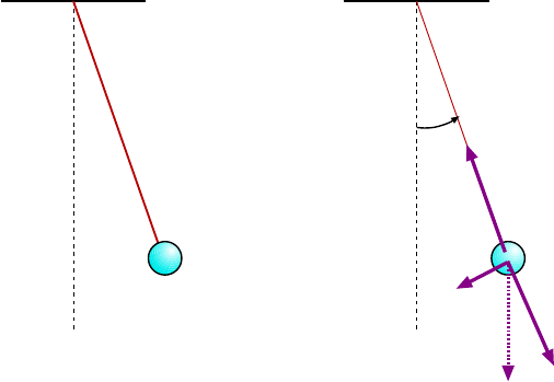
146 CHAPTER 10. OSCILLATORY MOTION
m
L
q
0
m
q
(a)
(b)
mg
mg cosq
mg sinq
T
Figure 10.9: (a) Simple pendulum o f length L with small mass m attached to the end. Pendulum is pulled
back by θ
0
and released. (b) Forces acting on the mass when pendulum is at angle θ from the vertical. The
down ward force of gravity mg has been split into components along and perpendicular to the string.
10. 1.7 Simple Pendulum
Another oscillating system is shown in Fig. 10.9(a). A small mass m is attached to a light
string of length `; it is pulled back by some angle θ
0
and released. The mass swings back
and forth in a vertical plane. This is a pendulum, of course; since all the mass in the system
is at the very end of the string it is called a simple pendulum.
Clearly the mass will swing back and forth between angles of ±θ
0
from the vertical.
(Total energy will remain the same so it will rise to the same height as when it started.)
We’d like to find how the period of this motion depends on the physical properties of the
pendulum.
We can view the mass and string as a system that rotates about the place where the
string is attached. Then since t here is only a single point mass a distance L f r om the axis,
the moment of inertia of this system is I = mL
2
.
The torque on the system is provided by grav ity. The forces acting on the mass are shown
in Fig. 10.9(b). String tension T pulls inward along the string’s length and the downward
force of gravity, mg has been split up into components along the string and perpendicular to
it. The forces which act along the string give no torque about the axis (the sin φ factor for
the torque is zero) but the perpendicular part of gravity, mg sin θ is exerted at a distance of
L and gi ves a torque of magnitude τ = L(mg sin θ).
We ne ed to get the sign of the torque correct here. From Fig. 10.9(b) we see that when
θ is positive, the torque τ is in the opposite (negative) sense, so actually we should say :
τ = −mgL sin θ
10.1. THE IMPORTANT STUFF 147
From τ = Iα and I = mL
2
we then get
τ = −mgL sin θ = (mL
2
)α
and the n some algebra gives
α = −
g
L
sin θ (10.11)
One more step is needed so that we can get f from this eq uation. It turns out that when
the angle θ is small (and measured in radians, as is assumed in Eq. 10.11) the value of sin θ
is very close to the value of θ itself. If θ is less than the radian equivalent of 20
◦
the two
values are within 2% of each other. We will promise (hah!) never to use our results when
the angle of swing is greater than 20
◦
and then in place of Eq. 10.11 we will write
α = −
g
L
θ (10.12)
Now we recal l the eq uations for the mass and spring. We had F
x
= −kx and F
x
= ma
x
.
Combining these equations gives:
a
x
= −
"
k
m
#
x (10.13)
an equation which is similar in form to Eq. 10.12.
Now from Eq. 10.6 we found that ω
2
for the mass–spring system is k/m, namely the
thing inside the square brackets in Eq. 10.13. It is sensible (and valid) to conclude that ω
2
for the simple pendulum is the thing i nside the brackets in Eq. 10.12. So for the pendulum
system we have:
ω
2
=
g
L
=⇒ ω =
r
g
L
(10.14)
and the n from f = ω/(2π) we have
f =
1
2π
r
g
L
(10.15)
and using T = 1/f we get the period of the pendulum,
T = 2π
s
L
g
(10.16)
The result for f (or T ) is surpri sing because of what is not in the formula. The mass of
the pendulum bob is not there; as long as the mass is great enough so that air resistance is
not significant the period is the same for any small b ob attached to the end.
Secondly, the i nitial angle θ
0
does not appear. Does this mean that the period of a
pendulum does not depend on how far back you pull it initially? Pretty much, yes. But
we must recall that we are alway s working within the approximation that all the angles are
“small”! If you pull the pendulum back by 60
◦
there will be a significant (i.e. measurable)
difference from the perio d you get by starting the pendulum at 5
◦
.
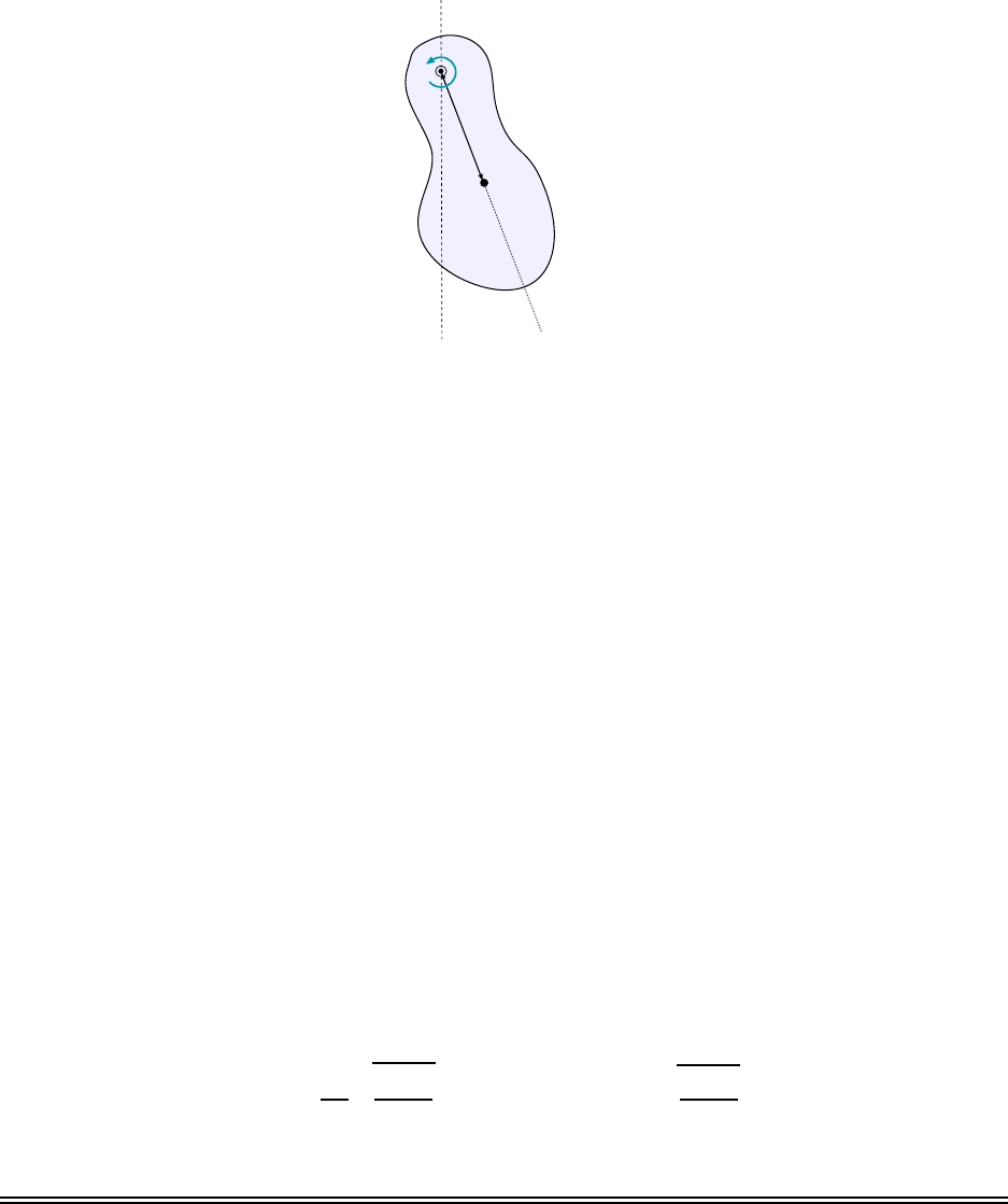
148 CHAPTER 10. OSCILLATORY MOTION
CM
L
M
q
Mom. of Inertia = I
Figure 10.10: A “physical” pendulum . (What pendulum is not physical??) Object has moment of inertia
I about the pivot; center of mass is a distance L from the pivot.
10. 1.8 Physi cal Pendulum
For completeness, we give t he results for a different kind of pendulum, but one which you
may encounter in your problem sets or in the lab.
Suppose we suspend an object by a frictionless pivot so that its center of mass hangs
below this pivot. Then we give the object a small displacement from the vertical position
and let it oscillate back and forth.
Such an object is a kind of pendulum, but not a simple one bec ause its mass is not
concentrated at one p oint. People usually cal l it a physical pendulum, but I have yet to
see a pendulum which is not “physical”.
Hey, I just work he re.
Anyway, when we write down the equations for the torque and angular acceleration of this
object (similar to what we did above for the s i mple pendulum) we find that the frequency of
the moti on depends on the total mass M of the object, the moment of inert ia of the object
about the pivot point I and the distance L fr om t he pivot to the center of mass of the object;
see Fig. 10.10. Recall that to get the moment of inertia about points other than the center
of mass the parallel axis theorem (Eq. 9.5) can be helpful.
The result for the frequency and period is
f =
1
2π
s
MgL
I
and T = 2π
s
I
MgL
(10.17)
10.2. WORKED EXAMPLES 149
10.2 Worked Examples
10. 2.1 Harmonic Mo tion
1. Atoms in a solid are not stationary, but vibrate about their equilibrium
positions. Typically, the frequency of vibration is about f = 2.0 ×10
12
Hz, and the
amplitude is about 1. 1 × 10
−11
m. For a typical atom, what is its (a) max imum
speed and (b) maximum acceleration? [CJ7 10-15]
(a) The angular frequency of the atoms’ oscillations is
ω = 2πf = 2π(2.0 × 10
12
s
−1
= 1.26 × 10
13
s
−1
so using Eq. 10.4 the maximum speed of atom is
v
max
= ωA = (1.26 ×10
13
s
−1
)(1.1 × 10
−11
m) = 1.38 × 10
2
m
s
(b) U sing Eq. 10.5, the maximum acceleration of t he atom is
a
max
= ω
2
A = (1.26 × 10
13
s
−1
)
2
(1.1 × 10
−11
m) = 1.66 × 10
15
m
s
2
10. 2.2 Mass–Spring System
2. A 0.200 kg mass hanging from the end of a spring is set into motion. It is
found that the mass bobs up and down through 10 cycles in 6.50 s. What is the
force constant of the spring?
Find the period of the motion. Since 6.50 s was the time for ten cycles, we get :
T =
(6.50 s)
(10.0 cycle)
= 0.650 s
Then use Eq. 10.8 to solve for T :
T = 2π
r
m
k
=⇒ T
2
=
4π
2
m
k
=⇒ k =
4π
2
m
T
2
Plug in stuff:
k =
4π
2
(0.200 kg)
(0.650 s)
2
= 18.7
kg
s
2
= 18.7
N
m
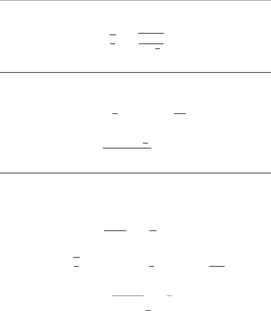
150 CHAPTER 10. OSCILLATORY MOTION
10. 2.3 Simple Pendulum
3. What is the period of a simple pendulum which has a length of 3.00 m?
Use Eq. 10.16 with L = 3.00 m. Get:
T = 2π
s
L
g
= 2π
v
u
u
t
(3.00 m)
9.80
m
s
2
= 3.48 s
The period of the pendulum is 3. 48 s.
4. What is the length of a simple pendulum which has a period of 1.00 s?
Use Eq. 10.16; square both sides then solve for L. We get:
T
2
= 4π
2
L
g
=⇒ L =
T
2
g
4π
2
Plug in T = 1.00 s and get:
L =
(1.00 s)
2
(9.80
m
s
2
)
4π
2
= 0.248 m
A pendulum with a length of 0.248 m = 24.8 cm will have a period of 1.00 s.
5. A simple pendulum of length 2.0 m is being swung on the surface of some
strange planet . It makes 20 compl ete oscillations in 51.7 s. What is the value of
g on this planet?
To get the period of this pendulum, find the tim e per oscillation:
T =
(51.7 s)
(20 osc)
= 2.59
s
osc
= 2.59 s
Solve for g fr om Eq. 10.16:
T = 2π
s
L
g
=⇒ T
2
= 4π
2
L
g
=⇒ g =
4π
2
L
T
2
Plug in the numbers:
g =
4π
2
(2.0 m)
(2.59 s)
2
= 11.8
m
s
2
The acceleration of gravity on this planet is 11.8
m
s
2
.
Chapter 11
Waves I
11.1 The Important Stuff
11. 1.1 Introduction
A wave (as we’ll use the term in this chapter) is a disturbance in some continuous, deformable
and otherwise uniform medium whi ch travels over “long” distances whil e the little bits of
the medium itself are moving over relatively small distances. Familiar examples of waves
are the surface waves on water, the waves on a vibrati ng string and sound waves, which are
travelling distortions in the density of air.
Light and electromagnetic waves in general have some properties in common with these
types of waves, but electromagnetic waves are differe nt in that they do not travel through
any medium. Also, they arise from the electric and magnetic fields we’ll study later on, and
as such they are best left to that part of the course.
Wave phenomena occur around us all the time and if only for that reason it would be
important to study them. But it turns out that when we look at the behavior of matter
on the smallest scales, the basic ”particles” in nature don’t b ehave like particles following
Newton’s laws as presented in this course; rather, they are waves.
In the end, it’s all waves.
Waves are characterized by the direction in which the little bits of the medium move in
relation to the direction of motion of the wave itself.
For a wave on a taut string the elements of the string move perpendicularly to the direction
of propagation of the wave, as shown in Fig. — (a). Such a wave is called a tr ansverse
wave. These waves are the easiest to visualize.
For others, the motion of the medium is along the direction of propagation of the wave.
An example of this (one that can be seen, at least) is that of a Slinky which has been tapped
along its length. The disturbance which one sees travelli ng down the Sl inky is a region where
151
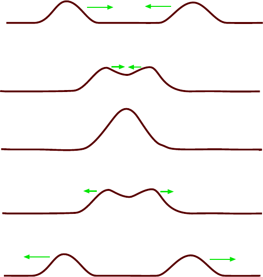
152 CHAPTER 11. WAVES I
(a)
(b)
(c)
(d)
(e)
Figure 11.1: Two “positive” pulses are put on a string; they travel towards one another, add constructively
and then continue on as if nothing had happened!
the coils are slightly compressed. This type of wave is called a longitudinal wave.
The waves (and the media through which they travel) which we’ll study will have the
property that the di sturbance will propagate unchanged.
11. 1.2 Principle of Superpos ition
Another prop erty of the waves (and media) which we’ll study is that individual waves “add
together”. What we mean by this is that if we have two sources of waves the wave that
is present when both sources operate at once is the sum of the waves that are present
when the sources are operating individually. We do mean the literal sum here; we add the
displacem ents of the medium at each p oint of the medium.
The idea of adding waves together is called the principle of superposition and it is obeyed
by all the media and waves that we will consider.
An example is gi ven in Fig. 11.1, something which you and a friend could demonstrate
with a rope, but you’d have to observe it very quickly! Here two pulses are put onto a rope
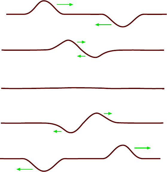
11.1. THE IMPORTANT STUFF 153
(a)
(b)
(c)
(d)
(e)
Figure 11.2: “Positive” and “negative” pulses of similar shape are created on a string and travel toward
each other. When they overlap the pulses cancel such that the rope is nearly fla t at some point. Then the
pulses emerge and keep on travelling.
by some sources, like the hands of the people holding the rope. The pulses travel toward one
another meet and continue onward after they meet. The displacements of the rope making
the pulses are in the same direction for the two pulses. When the pulses meet at the ce nter
their displacements add together to give a larger pulse. Somehow the rope “knows” that it
contains two individual pulses so that the pulses again separate and keep moving in their
original directions!
I k id you not, this really happens.
When waves combine so that the resulting wave is “larger” than the individual waves,
we say that constructive interference is taking place.
Even stranger is when the two people holding the rope create travelling pulses with
opposite displacements, i.e. for one pulse the string disturbance goes “up” while for the
other it goes “down”, as shown in Fig. 11.2. When the pul ses begin to overlap the sum
of the waves has a smaller size than the individual wave and we say that destructive
interfere nce is taking place . When the waves precisely overlap the string is very nearly
flat! (We assume the two pulses had similar shapes.) Nevertheless, an instant later the two
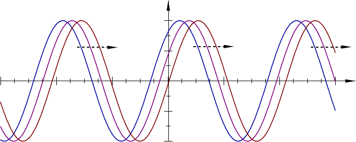
154 CHAPTER 11. WAVES I
-3 -2 -1 0 1 2 3
Figure 11.3: A harmonic wave is a sinusoidal pattern that travels to the left or right.
pulses emerge and continue on thei r separate ways.
How can this be? If the string is mome ntarily flat, haven’t the two waves been “killed”?
Then why do the pulses reappe ar? What you don’t see in Fig. 11.2(c) is the instantaneous
velocity of the parts of the string and these are not zero. The “memory” of the shapes is
contained in that movement and when we wait a little longer we get t he two pulses back
again.
11. 1.3 Harmonic Waves
Things could get mighty complicated if we were to consider waves of any shape whatsoever.
It turns out that if we focus on a particular kind of wave with a repeating pattern of
displacem ent we will know about all we need to know about waves. Some of the reasons are
“beyond the scope of the course” as they say, but it’s al so true that many wave sources will
produce a r epe ating pattern and then our results wi ll be useful for describing the real world.
The ki nd of wave we want to study i s shown in Fig. 11.3. It is sinusoidal in shape and is
essentially infinite in length. And since it is a wave, it is moving in some direction, ei ther to
the l eft or to the right with some speed v.
Can you visualize that? I hope so. . . if only I could put an animated picture of the wave
onto this page! M aybe in the future the pages of books will be able to show moving pictures.
For now we’re stuck with paper and still pictures. So you’ll have to imagine that the pattern
in Fig. 11.3. is moving to the ri ght.
Such a wave is called a harmonic wave.
Again, using your imagination think of the moving sinusoidal pattern as a wave on a
string and consider the motion of any single point on the string. A single poi nt j ust m oves
up and down, much like a harmonic oscillator in the previous chapter; see F ig. 11.4. In fact
for the harmonic wave, the motion of a single point is exactly that of a harmonic oscillator;
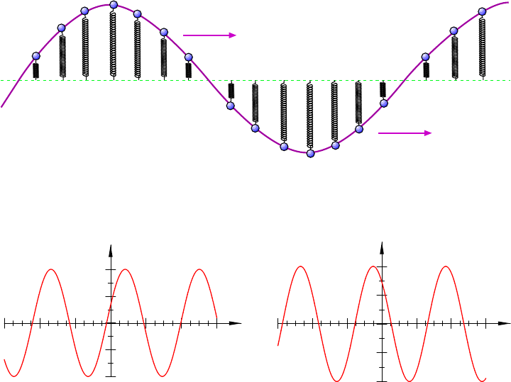
11.1. THE IMPORTANT STUFF 155
Figure 11.4: The individual points on the harmonic wave act like harmonic oscil lators, moving up and
down.
A
A
y
y
x
t
-A
-A
(b)
(a)
Figure 11.5: (a) At a fixed time t the displacement y has a sinusoidal dependence on the coordinate x.
(b) At a fixed location x the displacement has a sinusoidal dependence on the time t.
it is sinusoidal in its time dependence also.
The harmonic wave is sinusoidal in a double sense: Freeze the time and the wave is
sinusoidal in x. Fix the location x and the wave is sinusoidal in the time t. This is shown in
Fig. 11.5.
Damn, I wish I could put animated pictures in a book.
Two important numbers which characterize a harmonic wave are the wavelength and the
frequency. In Fig. 11.6 we show a picture of a harmonic wave “frozen” at some particular
time t. The length of string from any place on the wave to where it starts to repeat is the
wavelength of the wave. It is usuall y given the symbol λ and is measured in meters (since
it is a length!).
Next we think of t he motion of an individual bit of the string (li ke the individual elem ents
shown in Fig. 11.4). A plot of its di splacement versus time might look like Fig. 11.7. The
string element oscillates up and down and therefore its m otion has a frequency, just like the
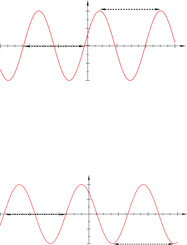
156 CHAPTER 11. WAVES I
λ
x
λ
-A
A
y
Figure 11.6: When we “freeze” the time t, the wavelength λ is the length along the string for one full cycle
of the displacement.
y
t
-A
A
T
T
Figure 11.7: When we choose a bit of the string a t a particular x, the period T is the time needed for one
full cycle of the displacement. The frequency of the wave is given by f = 1/T .
11.1. THE IMPORTANT STUFF 157
oscill ators in the last chapter. This is what we mean by the frequency of the wave. The
frequency (f) is measured in Hz=
cycle
s
.
And now we want to think about the space and time dependence of the wave simultane-
ously. If you can really visualize the wave motion (and it is a bit tricky) you can see that
in the time T (the time in whi ch one bit of the stri ng moves through a full cycle) the wave
moves forward by one wavelength, i.e. in a time T the waves moves forward a distance λ.
That m eans that the speed of the wave (v) is given by:
v =
λ
T
But since T = 1/f this gives us
v =
λ
(1/f)
= λf ,
that is,
λf = v (11.1)
11. 1.4 Waves o n a String
The speed of waves on a string depends on the tension (called F here) and the “bulkiness”
of the string material, which is given by the mass per unit length of the string. For a string
of length L and mass m under tension F i t is given by:
v =
s
F
(m/L)
=
s
F
µ
(11.2)
where µ = m/L.
11. 1.5 Sound Waves
A sound wave is a longitudinal wave in the density of some medium; most often we consider
the atmosphere as the medium but it could be a liquid or solid. Fluctuations in the density
of the medium occur because of the tiny motions of the elements of the medium (the atoms
and molecules) along the di r ection of moti on of the wave.
Because of the collective motions of the molecules there are regions where the density is
slightly greater or less than the “normal” density of the medium and it is these regions of
greater or lesser density which from the disturbance which travels, i.e. t he sound wave. An
exaggerated pi cture is shown in Fig. 11.8. Again, the problem with such still pictures i s that
they don’t show the motion of the wave or how the high/low density regions are formed by
the moti ons of the littl e bits of the medium.
I wish I knew how to put animated pictures in these notes! Then it would look good.
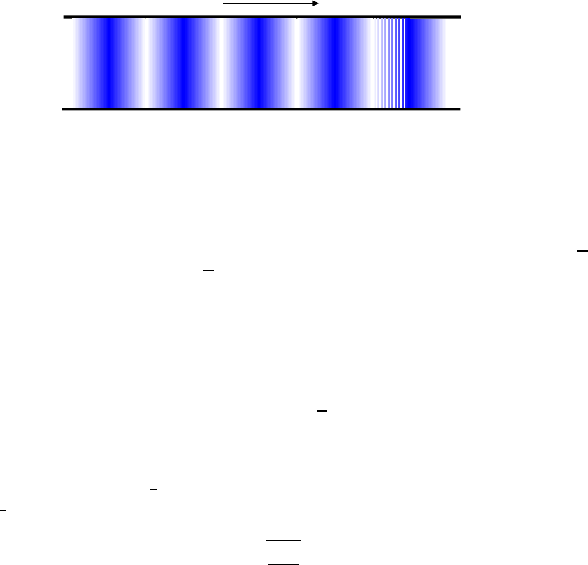
158 CHAPTER 11. WAVES I
v
Figure 11.8: Sound wave travels down air a ir-filled pipe with speed v.
Damn.
Anyway, the speed of sound is strongly dependent on the type of medium in which the
wave travels. Even for sound waves in air at normal pressure the speed depends si gnificantly
on the temperature of the air: In air at at 1 atm of pressure and at 20
◦
C the speed is 343
m
s
but at a temperature of 0
◦
C it is 331
m
s
.
There is actually a formula for t he speed of sound waves in a gas. It involves some
quantities not covered yet in these notes but it is useful to write it down here. Suppose
the absolute (Kel vin) temperature of the gas is T and the mass of one of its m olecules is
m. There is a numbe r important is the study of the thermal properties matter called the
Boltzmann co nstant, k which is given by:
k = 1.38 ×10
−23
J
K
Finally there is a unitless number symbolized by γ which is characteristic of the type of
molec ules in the gas and some other factors; for monatomic gases under “normal” (room
temperature) conditions it is
5
3
; for diatomic gasses (li ke those in the atmosphere, N
2
and
O
2
) it is
7
5
. Anyway, with all of this, the speed of sound is given by
v =
s
γkT
m
(11.3)
11. 1.6 Sound Intensity
The two important aspects of a sound wave are its f requency (if it is a harmonic wave)
and its amplitude (i.e. it s loudness). Si nce in a sound wave the particles of the medi um
oscill ate back and f orth (on average) along the direction of propagation we could talk about
a displacement amplitude for the sound wave. Likewise, since the wave is formed of
pressure variations along the direction of propagation, one could also speak of a pressure
amplitude for the wave. These two type of amplitudes are related, but we won’t discuss
them f urther; refer to more complete physics text s.
11.1. THE IMPORTANT STUFF 159
v
v
v
v
Figure 11.9: Spherical wave.
It is more useful to desc r ibe the loudness of a sound wave in terms of the rate at which it
transports energy. At a large distance from a source of sound, the wave maxima are close to
a set of equally spaced planes moving forward at speed v. If we consider a planar surface of
area A through the wave passes then in a time t the wave will tr ansfer an amount of ene r gy
E; E is clearly proportional to both A and t, so dividing them out gives a measure of the
strength of the sound wave, its intensity:
I =
E
At
(11.4)
The intensity I has units of
J
m
2
·s
, or
W
m
2
.
The human ear can detect sounds with a large range of intensities, from 10
−12
W
m
2
(the
threshold of hearing) to 10
W
m
2
, for which t he sound wave is intense enough to be harmful. It
is useful to have a measure of i ntensity which gives the order of magnitude of the intensity,
and such a measure is given by the intensity le vel, defined by:
β = (10 dB) log
10
I
I
0
(11.5)
where I
0
= 10
−12
W
m
2
. The intensity level β has units of decibels, or dB.
Sometimes, a useful approximation in dealing with sound waves is to imagine that the
wave was created by a source that makes a wave go out radially, that is, equally is all
direct ions. This is the approximation of an isotr opic source , and t he wave from such a
source is illustrated in Fig. 11.9.
Such a source will put a certain amount of power P into the generation of the wave and
this energy is transmitted outward in all direc t ions. If we consider a spherical surface of

160 CHAPTER 11. WAVES I
radius r centered on the source then the rate at which energy crosses this surface is also
P . The energy flux at this distance can then be found by taking the total power crossing
the surface (P ) and dividing by the total area of that surface (4πr
2
). Then the intensity of
sound waves at distance f r om an isotropic source of power P is
I =
P
4πr
2
(11.6)
11. 1.7 The Do ppler Effect
An interesting effect occurs when a source of sound (isotropic, for simplicity) i s in motion
through the medium through which the sound travels (usuall y the air, which we take to be
“stationary”). In Fig. — we show a source in motion toward an observer. The source has
speed v
s
and here the observer is at rest with re spect to the air.
We see that since the waves were emitted from different points (due to the motion of the
source) the wave maxima (indic ated with the circles) are bunched up in front of the source,
that is, more bunched up than if the source were standing still. Likewise, they are more
separated behind the source.
In this case, the observer will receive waves which are travelling at the usual speed but
which effectively have a shorter wavelength. Then the frequency of the wave must be larger
than if the source were standing sti ll. One can show that the observer would hear a freque ncy
f
o
given by
f
o
= f
s
1
1 −
v
s
v
!
where v is the speed of sound (in air), f
s
is the frequency of the source and v
s
is the speed
of the source toward the observer.
Conversely, if the observer had been behind the source, s/he would hear a frequency
lower than if the source were standing still and it would b e given by
f
o
= f
s
1
1 +
v
s
v
!
The two formulae can be combined as:
f
o
= f
s
1
1 ∓
v
s
v
!
(11.7)
where we take the bottom sign for motion of source toward the observer
There will also be an change in the frequency re ceived from a source is the source i s
stationary but the observer is in motion. Fig. — shows an observer running toward a source
of sound. In this case, the spacing of the wave maxima has its normal value, but the observer
11.2. WORKED EXAMPLES 161
encounters the wave maxima at a greater rate b ecause of his motion. In effect, the speed of
the waves is greater and so again the observer hears a larger frequency.
If the observer had been running away from the source he would have heard a lower
frequency.
The result for the two cases can be combined into one formula as:
f
o
= f
s
1 ±
v
o
v
(11.8)
where as before we take the bottom sign for motion of the observer t oward the source.
If both the source and observer are in motion the n we must have to use the most general
formula, which is basically a combination of Eqs. 11.7 and 11.8:
f
o
= f
s
1 ±
v
o
v
1 ∓
v
s
v
!
(11.9)
where the choice of sign is the top one for “toward” and the bottom one for “away”.
11.2 Worked Examples
11. 2.1 Harmonic Waves
1. A harmonic wave on a string has a spe ed of 220
m
s
and a wavelength of 0.720 m.
What is the frequency of the wave?
Use Eq. 11.1 and solve for f:
λf = v =⇒ f =
v
λ
Substitute for v and λ and get:
f =
(220
m
s
)
(0.720 m)
= 306 Hz
The freq uency of the wave is 306 Hz.
Note that even though the units come out as “
1
s
” here, a frequency should be expressed
in units of
cycle
s
= Hz.
162 CHAPTER 11. WAVES I
2. What is the wavelength of a harmonic wave on a string if the speed of the
waves is 160
m
s
and the frequency of the wave is 220 Hz?
Use Eq. 11.1 and solve for λ; plug in the numbers and get
λ =
v
f
=
(160
m
s
)
(220
cycle
s
= 0.727 m
11. 2.2 Waves o n a String
3. The linear density of the A str ing on a violin is 7.4 ×10
−4
kg/m. A wave on the
string has a freque ncy of 440 Hz and a wavelength of 65 cm. What is the tension
in the string? [CJ6 16-13]
We are given the values of λ and f for this string wave so from Eq. 11.1 we ca get the
speed of the wave:
v = λf = (0.650 cm)(440 s
−1
) = 286
m
s
Eq. 11.2 relates the wave speed v to the tension F and mass density µ; solve for F :
v =
s
F
µ
=⇒ v
2
=
F
µ
=⇒ F = µv
2
Plug in:
F = (7.4 × 10
−4
kg
m
)(286
m
s
)
2
= 60.5 N
11. 2.3 Sound Waves
